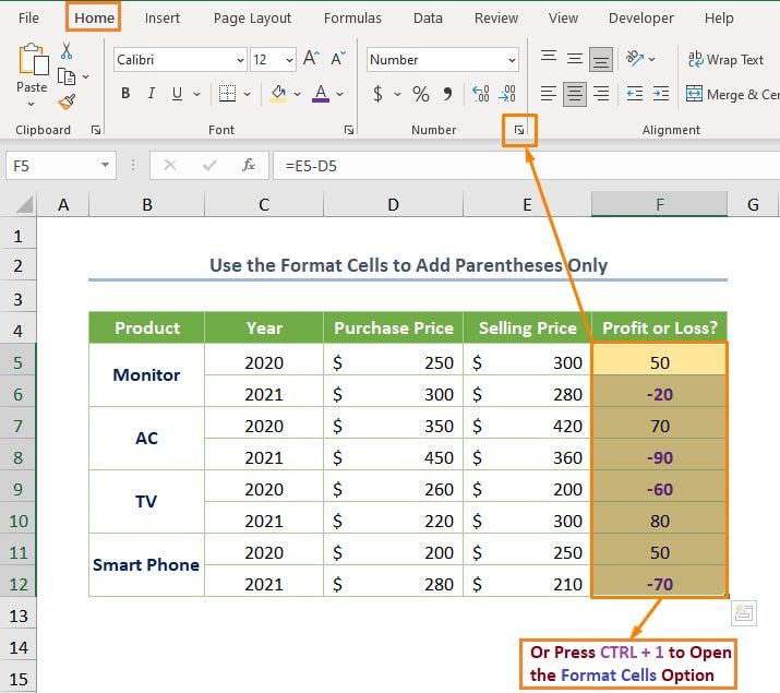
Display Negative Numbers in Excel Parentheses (Brackets) (Easy Ways)

Excel enables you to display numbers in a variety of formats because it is used by people across all sectors and professions.

Showing negative numbers in brackets is a typical number format that must be utilised when working with financial data and producing accounting reports (parentheses).

Although negative numbers in Excel are typically displayed with a minus sign, it’s simple to change the format to display negative values in brackets or parentheses.

I’ll demonstrate many methods for putting negative values in brackets in this article. I’ll also go over all the various formatting choices you have (such as adding or removing the – or changing the color of the negative or positive numbers)

This instruction explains:

Display Negative Numbers using In-Built Formats
Create a Custom Format to Display Negative Numbers in Brackets
Number Format: Why Isn’t the Parenthesis Option Visible? What to Do!

Display Negative Numbers using In-Built Formats:

Several built-in number formats in Excel already display the negative number in brackets.

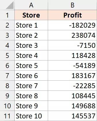
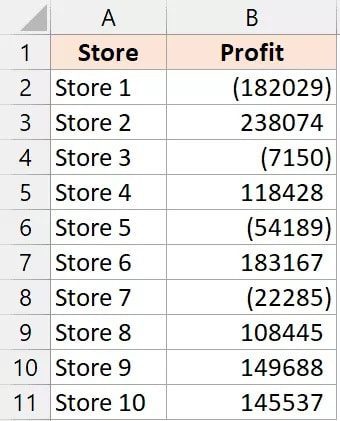
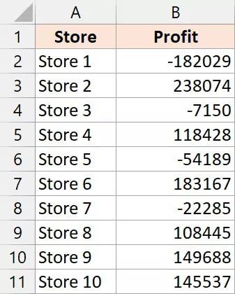
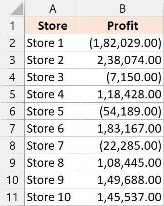
Column B of the data set below contains the profit figures for various stores, and I want to display the negative values in brackets.

The steps are as follows:

Choose the cells that contain numbers (you can select the entire range of cells, not just the negative numbers)
Choose the “Home” tab.

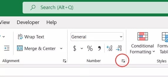
3. Click on the icon for the dialogue box launcher in the ‘Number’ group (small arrow at the bottom right part of the group)

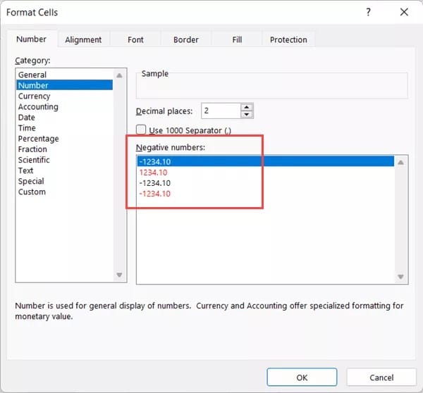
4. Choose the third option from the Negative Numbers list in the “Format Cells” dialogue box’s “Number” tab (the one that shows the number in the bracket as is in black color)

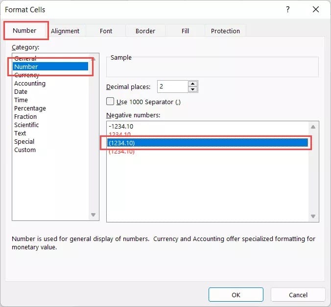
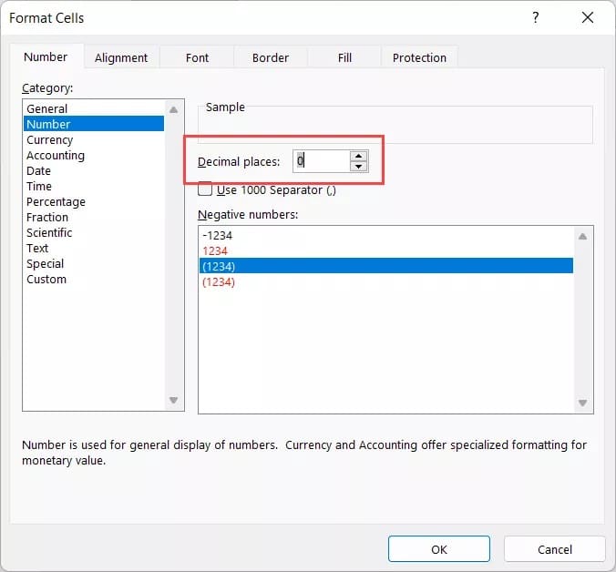
5. [Optional] Name the decimal numbers you want displayed. Make the value 0 if you don’t want decimal numbers (it is 2 by default).

6. Input OK.

The aforementioned actions would modify the cells’ formatting so that negative integers are now shown in parenthesis (as shown below).

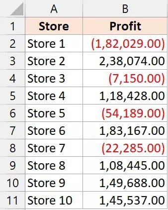
Additionally, you have the choice to put negative integers in brackets and change their colour to red in the “Format Cells” dialogue box.

Choose the fourth option in step 4 to display negative numbers in red within brackets.

‘You might not have access to the formatting options for “Negative numbers” I’ve displayed in the screenshots above. Some system configurations disable the option to format negative integers, so they appear in brackets. The alternatives are instead indicated with a negative symbol. If so, you will need to modify your system settings, which will be explained in more detail later in this article’.

Create a Custom Format to Display Negative Numbers in Brackets:

While the aforementioned approach does allow you to display negative numbers in brackets (in a black or red colour), you may also design your own unique number format if you require greater control over how these numbers are displayed.

For instance, you could want to display the negative numbers with a minus sign and in brackets (or alternatively, by painting them orange or brown rather than red).

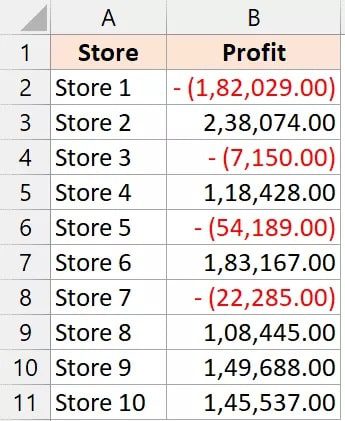
I have a dataset with negative numbers in it that I want to display with the minus sign and the negative values enclosed in brackets.

The procedures are as follows:

Select the cells you want to format that contain negative integers.
Choose the “Home” tab.
To open a dialogue box, select the “Number” group’s launcher.
Choose the “Custom” option from the “Number” tab of the “Format Cells” dialogue box.

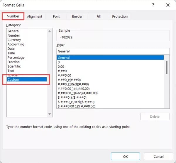
5. Enter the custom format shown below in the “Type” field.

0;- (0)

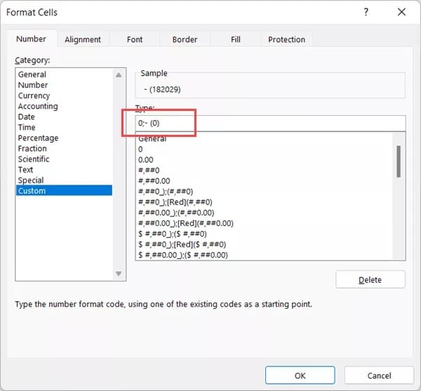
6. Input OK.

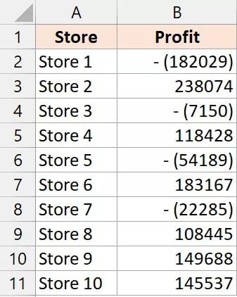
The formatting of the cells would be altered as a result of the aforementioned processes, and negative integers would now be displayed in brackets with a minus sign.

Before I offer you some examples of alternative formats you can use, let me briefly explain how custom number formatting functions.

You can enter the following kinds of data in Excel:

Positive Number
Negative Number
Zero
Text

You can specify the format for any of the aforementioned data types for any cell. This entails that I may specify how text values and zeroes should be shown, as well as how positive and negative numbers should be displayed in a cell.

And here is how you should build the custom number format:

<Format for Positive Number>;<Format for Negative Number>;<Format for Zero>;<Format for Text>

Keep in mind that a semi-colon separates each of these formats.

Any of these four data types would utilize the ‘General’ format if the format is not specified.

In our illustration, we choose the format 0;- (0)

Where:

Positive Number Format – 0 – This indicates that the entered number should be shown.

Negative Number Format – – (0) – This instructs the display of the number as it was input inside the parentheses.

Zero Format – this will be interpreted as General because it is not stated.

Text format will be assumed to be General because it is not specified.

In this instance, any negative number would be displayed in a bracket with a negative sign outside the bracket because we have set the format for negative numbers to be – (#,##0).

Here are some additional formats you may use now that you have a basic idea of how custom number formatting in Excel works:

placing negative numbers in parentheses and using thousand separators to display numbers

#,##0.00;(#,##0.00)

displaying the negative figures in parenthesis and in red

#,##0.00;[Red](#,##0.00)

Displaying the negative numbers in parenthesis with a minus sign and in red:

#,##0.00;[Red]- (#,##0.00)

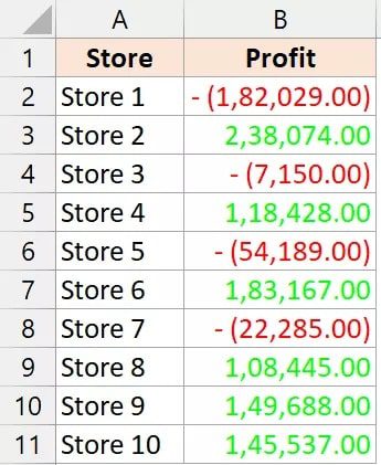
Showing the positive numbers in green and the negative ones in red

[Green]#,##0.00;[Red]- (#,##0.00)

Number Format: Why Isn’t the Parenthesis Option Visible? What to Do!

The option to display negative numbers in brackets appears when you open the Format Cells dialogue box and choose the Number option (as shown below).

If you don’t see these choices, it can be due of your system’s settings.

In order to format cells so that negative integers are displayed inside parenthesis, you can adjust the settings as follows:

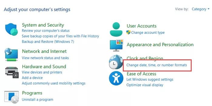
On your computer, launch Control Panel.
To change the date, time, or numeric formats, select that option.

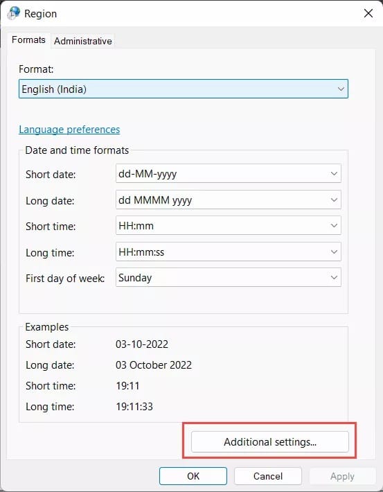
Click the “Additional Settings” option in the Region dialogue box.

Modify the format of the negative numbers under the Numbers tab (from the drop-down)

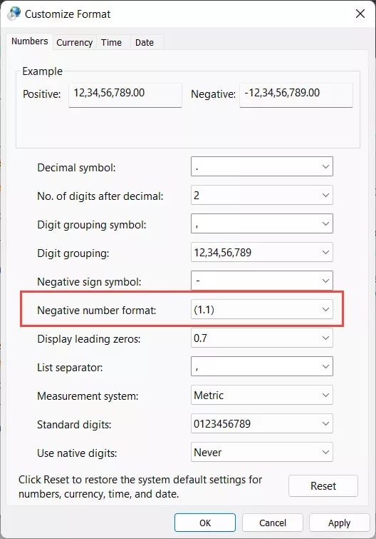
5. Input OK.

6. Input OK.

By following the instructions above, you can modify your system’s settings and access the formatting option to display negative integers in brackets in the Format Cells dialogue box.

I demonstrated in this lesson how to modify the cell’s format so that negative integers are displayed in brackets. I also went through how to modify the color of the negative numbers and add a minus sign in addition to the brackets in the format.