Skip to content
 How to Get Rid of Leading Zeros in Excel (5 Easy Ways)
Leading zeros in Excel are something that many people either love or loathe.
You don’t always want it, but sometimes you do.
Even though Excel is built to automatically remove any leading zeros from the numbers, there are few situations when you could still have them.
I’ll demonstrate in this Excel lesson how to get rid of leading zeros in your figures.
Then let’s get going!
This instruction explains:
1. Potential Causes of Leading Zeros in Excel 2. How to Clean Up Numbers of Leading Zeros 2.1 Make Numbers Out of Text by Using the Error Checking Option 2.2 Modify the Cells' Custom Number Formatting. 2.3 Increase by 1 (using Paste Special technique) 2.4 Making use of the VALUE function 2.5 How to Use Text to Columns 3. How to Clean the Text of Leading Zeros
1. Potential Causes of Leading Zeros in Excel
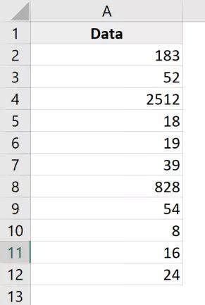
As I have said, Excel automatically strips numbers of any leading zeros. For instance, Excel will automatically change the value entered into a cell from 00100 to 100.
Most of the time, this makes sense because these leading zeros don’t imply anything.
But occasionally, you might desire it.
Your numbers can still have leading zeros for the following reasons:
- The preceding zeros would remain if the number had been treated as text, usually by placing an apostrophe before the number.
- It’s possible that the format of the cell was chosen such that a specific length of a number is always displayed. Additionally, leading zeros are appended to the integer to make up for any lower numbers. You may format a cell, for instance, to always display 5 digits (and if the number is less than five digits, leading zeros are added automatically)
Depending on the cause, we may use one of many methods to get rid of the leading zeros.
Therefore, the first step is to determine the cause so that we may pick the appropriate strategy to get rid of these leading zeros.
2. How to Clean Up Numbers of Leading Zeros
The leading zeros of numbers can be removed in a variety of ways.
I’ll demonstrate five of them to you in this part.
2.1 Make Numbers Out of Text by Using the Error Checking Option
If the leading numbers are a result of someone adding an apostrophe before the numbers (to turn them into text), you may use the error-checking method to instantly turn them back into numbers.
The quickest way to remove leading zeros is probably this.
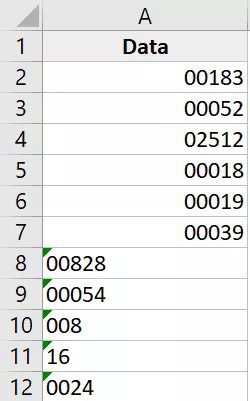
In this data collection, I have both the leading zeros and the numbers with an apostrophe before them. This is also the reason that these numbers contain leading 0s and are oriented to the left rather than to the right as is typical.
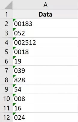
The procedures to eliminate these leading zeros from these integers are as follows:
Choose the numbers from which you wish the leading zeros removed. The upper right corner of the selection has a yellow symbol, as you will see.
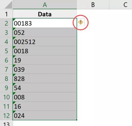
Tap the yellow error-checking icon.
Then select “Convert to Number.”
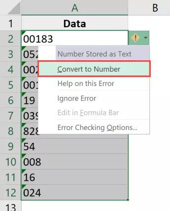
I’m done now! The apostrophe would be removed in the procedure above, and the text values would then be changed back to numbers.
The leading zeros are automatically removed when you do this since Excel is set up to eliminate leading spaces from all numbers by default.
Note: If the leading zeros were added as part of the cells’ custom number formatting, this solution would not function. Use the strategies discussed next to tackle those situations.
2.2 Modify the Cells’ Custom Number Formatting.
When your cells have been designed to always show a certain amount of digits in each number, this is another fairly typical reason why your numbers could appear with leading zeros.
Many individuals set the minimum length of the numbers by altering the cell formatting to make the numbers appear uniform and of the same length.
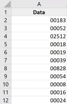
For instance, if you want all the numbers to display as five digits, Excel will automatically add two leading zeros to any values that are just three digits.
I’ve included a dataset with bespoke number formatting that always displays a minimum of five digits in each cell below.
Simply removing the present formatting from the cells will get rid of these leading zeros.
The procedures are as follows:
Choose the cells that include leading zeros in the numbers.
On the Home tab, click
Click the Number Format option in the Numbers group.
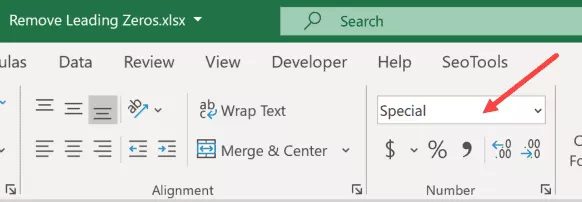
Choose “General”
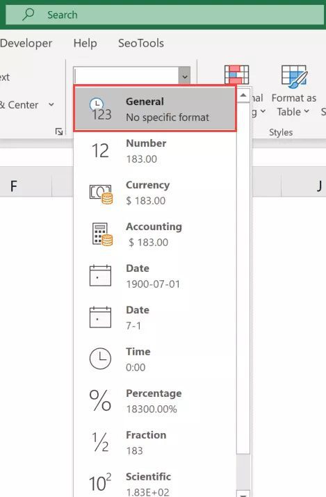
The aforementioned actions would alter the cells’ custom number formatting, and the numbers would then show as desired (where there would be no leading zeros).
Keep in mind that this method would only be effective if the leading zeros were being used for bespoke number formatting. If apostrophes were employed to convert numbers to text, it wouldn’t function (in which case you should use the previous method)
2.3 Increase by 1 (using Paste Special technique)
This method is effective in both situations (where the numbers have been converted into text by using an apostrophe or a custom number formatting has been applied to the cells).
Let’s say you wish to get rid of the leading zeros in the data set that is displayed below.
These are the procedures:
- Any blank cell on the worksheet can be copied.
- Choose the cells that contain the numbers you wish to delete the leading zeros from.
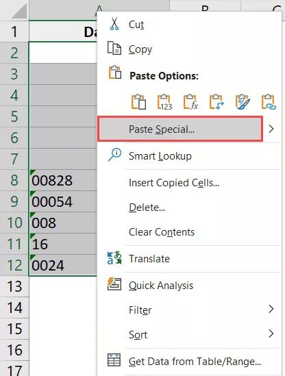
- Select the selection with the right click, and then select Paste Special. The Paste Special dialogue box will be shown.
- Click the “Add” button (in the operations group)
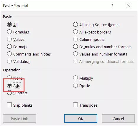
- Then OK
The aforementioned actions subtract all leading zeros and an apostrophe from the range of cells you specified and add 0 to it.
This preserves the cell’s value while converting all text values to numbers and copying the formatting from the blank cell you copied (thereby replacing the existing formatting that was making the leading zeros show up).
This approach solely affects the figures. If a cell has any text, it will remain there unaltered.
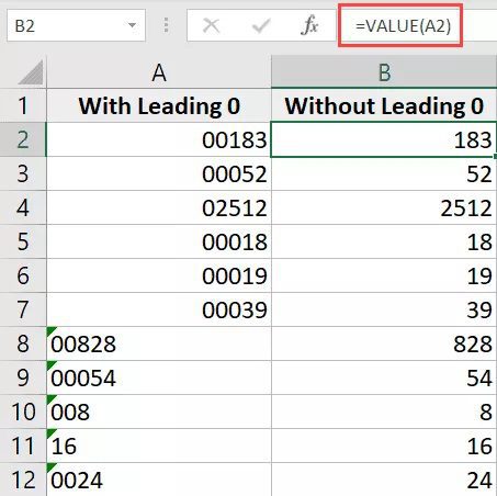
2.4 Making use of the VALUE function
Utilizing the value function is another quick and simple way to get rid of leading zeros.
The text or the cell reference containing the text may be used as the only parameter for this function, which returns the result as a number.
This would also apply in cases where your leading digits are the result of either bespoke number formatting or the apostrophe, which is utilized to transform numbers into text.
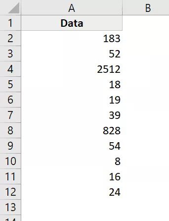
Let’s say I have the data set depicted below:

The equation to eliminate the leading zeros is as follows:
=VALUE(A1)
Note: If the leading zeros are still visible, switch the cell format to General on the home tab (from the Number Format dropdown).
2.5 How to Use Text to Columns
The Text to Columns feature may be used to eliminate the leading zeros in addition to dividing a cell into numerous columns.
Let’s say you have the data set depicted below:
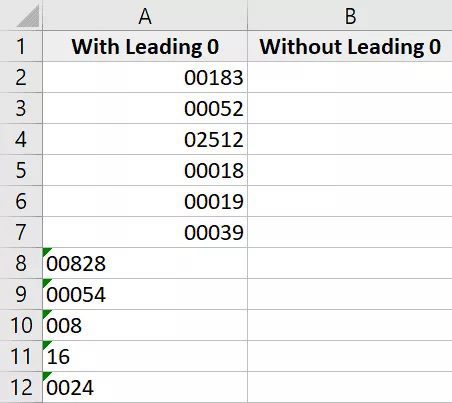
The procedures for eliminating leading zeros using Text to Columns are as follows:
- Choose the cells with numbers in them.
- Select the “Data” tab.
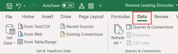
- Go to the Data Tools section and select “Text to Columns.”

- Changes need to be made in the “Convert Text to Columns” wizard as follows:
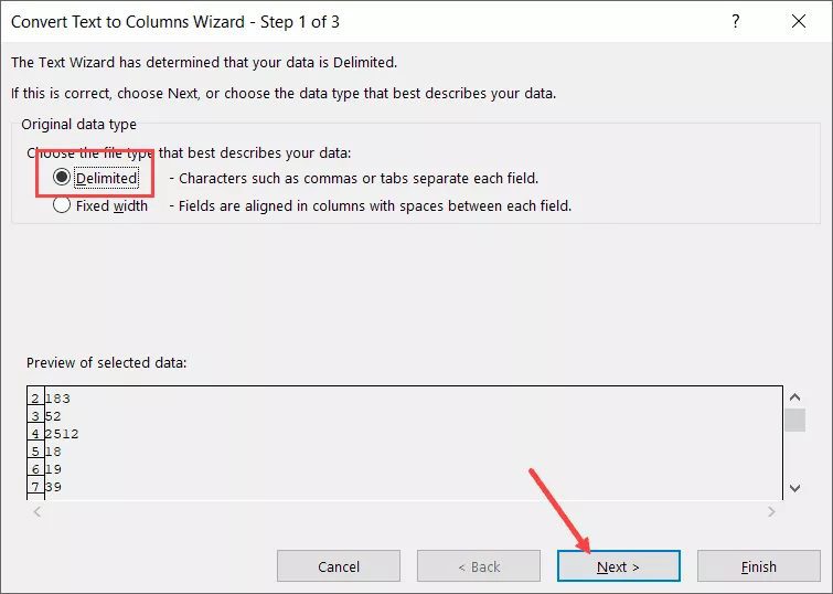
Step 1 of 3: Click Next after choosing “Delimited”
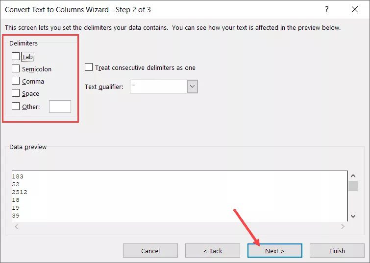
Step 2 of 3: Select None to deselect all delimiters, then select Next.
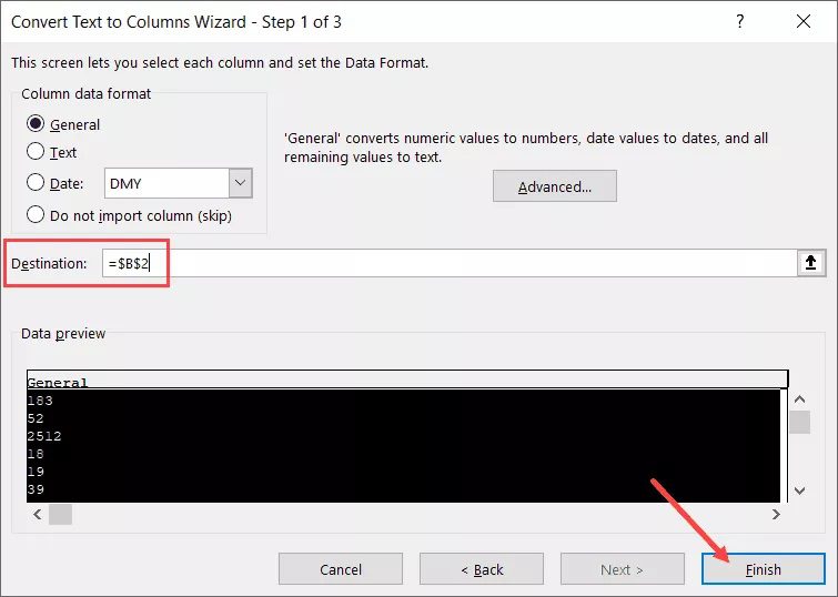
 Phase 3 of 3: Click on Finish after choosing a destination cell (in this case, B2).
The aforementioned methods ought to eliminate any leading zeros and leave you with only the numbers. If the leading zeros are still visible, you must switch the cells’ formatting to General (this can be done from the Home tab)
3. How to Clean the Text of Leading Zeros
All of the aforementioned techniques are excellent, but they are only intended for cells with a numerical value.
What happens, then, if your alphanumeric or text values also happen to contain some leading zeros?
In that situation, the aforementioned techniques would not be effective, but you can still acquire this time owing to Excel’s incredible formulae.
Consider the following data collection, which you wish to purge of all leading zeros:
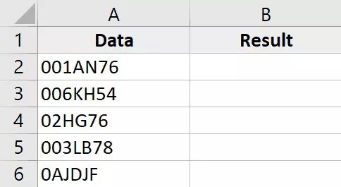
The formula to achieve it is as follows:
=RIGHT(A2,LEN(A2)-FIND(LEFT(SUBSTITUTE(A2,"0",""),1),A2)+1)
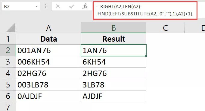
I’ll explain how this formula functions.
The formula’s SUBSTITUTE clause inserts a blank in lieu of the zero. As a consequence, the substitution formula returns 1AN76 as the result for the value 001AN76.
The LEFT formula then removes the first character from the resultant string, which in this instance would be 1.
The LEFT formula’s leftmost character is then searched for using the FIND formula, which then provides its location. In our case, it would result in 3 for the number 001AN76 (which is the position of 1 in the original text string).
To ensure that the complete text string is retrieved, 1 is appended to the FIND formula result (except the leading zeros)
Next, the outcome of the LEN calculation is subtracted from the outcome of the FIND formula (which is used to give the length of the entire text string). This provides us with the text ring’s length sans the leading zeros.
The RIGHT function is then applied to this value to extract the complete text string (except the leading zeros).
It is preferable to apply the TRIM function with each cell reference if there is a chance that your cells might have leading or trailing spaces.
As a result, the updated formula containing the TRIM function would look as follows:
=RIGHT(TRIM(A2),LEN(TRIM(A2))-FIND(LEFT(SUBSTITUTE(TRIM(A2),"0",""),1),TRIM(A2))+1)
These are a few simple techniques you may use to eliminate leading zeros from your Excel data file.
I sincerely hope this instruction was helpful.