Excel Unmerge Cells Instructions (3 Simple Methods + Shortcut)

There are several functionalities and tools in Excel. Some aspects are quite popular, but I wish they weren’t.

One such function is the capacity for cell merging.

Even though I don’t use it personally, I nevertheless frequently find myself unmerging cells (mostly in the workbooks shared by other people).

I’ll demonstrate a few fast techniques to unmerge cells in Excel in this article.

Although I don’t believe that cell merging will end anytime soon, I hope that these easy solutions to unmerge cells may help you save some time and pain.

This instruction explains:

1. Keyboard Shortcut for Cell Unmerging 2. Unmerge Cells Using the Ribbon's Option 3. Making the QAT's Unmerge Option available (One-click Unmerge) 4. Find each of the worksheet's merged cells. 5. Unmerge the cells and enter the original value in the empty cells.

1. Keyboard Shortcut for Cell Unmerging

Using a keyboard shortcut is the quickest way (at least for me) to unmerge cells in a worksheet.

You may either choose the entire worksheet and then unmerge all the merged cells from the entire sheet, or you can select a specified range of all the cells (from which you wish to unmerge cells).

The Excel keyboard shortcut for unmerging cells is listed below:

ALT + H M C

sequentially press each of these keys (one after the other).

All of the merged cells in the specified range would be instantaneously undone using the aforementioned shortcut.

When unmerging cells in Excel, you should keep the following in mind:

If there is text in the merged cells, it will move to the top-left cell in the set of merged cells that have been unmerged when you unmerge the cells.
Excel will combine all the cells if there are no merged cells in the selection. Control Z or just pressing the keyboard shortcut again will reverse this.

2. Unmerge Cells Using the Ribbon’s Option

Using the Merge & Center option on the ribbon is another, similarly quick method of unmerging cells in Excel.

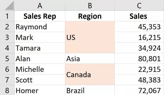
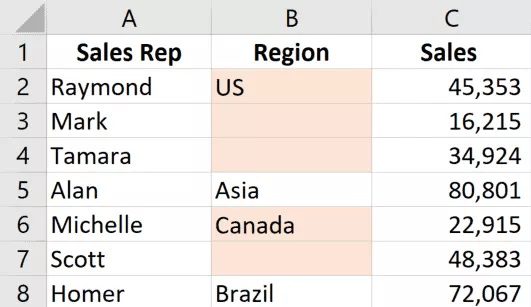
Let’s say you wish to undo the merging of the cells in Column B in the dataset depicted below.

The fast ways to unmerge these cells in Excel are listed below:

Choose the cells or the range of cells you wish to unmerge.
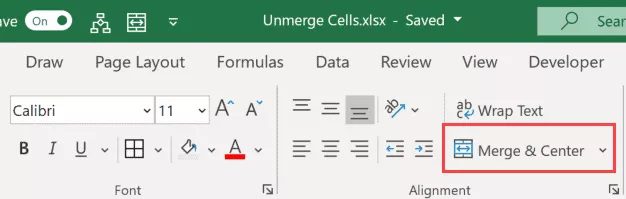
On the Home tab, click
Select “Merge & Center” by clicking the symbol in the Alignment group.

I’m done now!

All of the merged cells in the selection would be promptly undone by the aforementioned processes.

Keep in mind that the top cell now has the original value from the merged cells, leaving the lower cells empty.

This toggle button may also be used to combine cells (where you can simply select the cells that you want to merge and then click on this icon).

3. Making the QAT’s Unmerge Option available (One-click Unmerge)

Including the Merge & Center button in the Easy Access Toolbar is another quick method to unmerge sales in your spreadsheet (QAT).

In this manner, you may complete the task with a single click (as the quick access toolbar is always visible).

The procedures for adding the Merge & Center button to the quick access toolbar are as follows:

On the Home tab, click
Right-click on the ‘Merge and Center’ icon in the Alignment group.
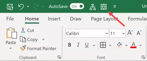
Select “Add to Quick Access Toolbar” from the menu. 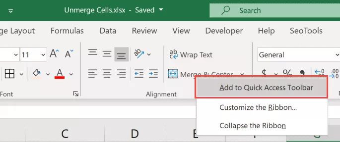The “Merge & Center” icon would be added to the quick access toolbar by following the procedures above. Simply make a selection and click on this button in the QAT to unmerge cells in Excel now.

Pro tip: You can also use a keyboard shortcut to reach an icon you’ve added to the Quick Access Toolbar. You could see a number underneath that icon if you held down the ALT key. Now, to use this keyboard shortcut, hold down the Alt key while pressing the appropriate number key.

4. Find each of the worksheet’s merged cells.

All of the techniques discussed up to this point would undo the merging of every cell in the selection.

However, what if you wanted to manually unmerge part of these merged cells? (and not all).

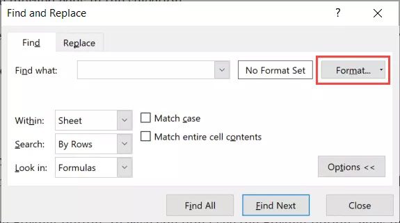
Excel’s “Find and Replace” tool may be used to rapidly locate all merged cells, pick just the ones you wish to undo the merging of, and then undo the merging of those cells.

The procedures are as follows:

Choose the range containing the cells you wish to unmerge.
Hold the Control key down while pressing the F key (or Command + F on a Mac) with the cells selected. The “Find and Replace” dialogue box will then be shown.
Tap the Format button in the Find and Replace dialogue box. If the Format button isn’t visible, click the Options button, and the Format button will appear.
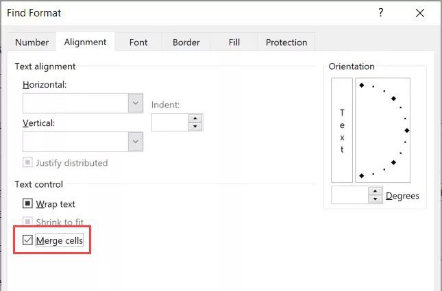
In the Find Format dialog box, click on the ‘Alignment’ tab
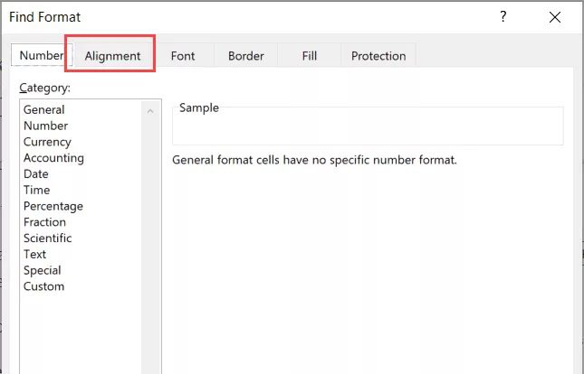
Select “Merge cells” from the menu.
Input OK.
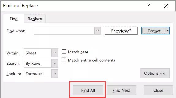
In the Find and Replace dialogue box, click the Find All button. This will locate all of the combined cells and display their cell references just beneath the dialogue box.
Select the cells you wish to unmerge manually while holding down the Control key.
To unmerge all of these cells, use the ribbon’s ‘Merge & Center’ option (or use any of the methods covered above)

Using this technique, you may selectively undo cell fusions while maintaining part of the original fused cells.

5. Unmerge the cells and enter the original value in the empty cells.

The value in the merged cell is assigned to the top-left cell when cells are unmerged in Excel, which is a problem (after the cells have been unmerged).

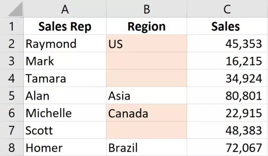
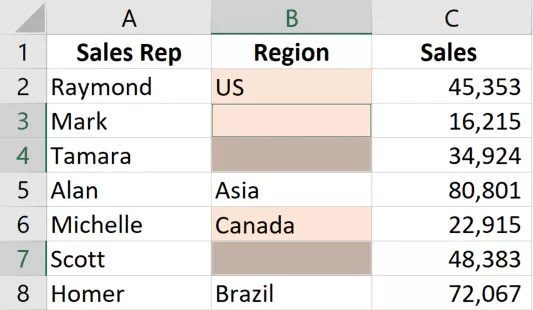
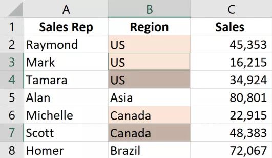
As a result, if you have a block of three cells that is merged and contains a value, unmerge the block to reveal the value in the top cell and leave the other two cells empty.

As you can see in the sample below, I have unmerged the cells (which are marked in orange), and all save the top cell are now empty.

How would you go about getting this value in each of these three cells?

This is simple to accomplish with a small workaround.

The steps to undo cell merging and fill every cell with its original value are as follows:

Choose the cells that were combined into one.
On the Home tab, click
Press the “Merge and Center” button under the Alignment group.
You will now have the unmerged cells, and you will notice that some of them are blank (which were earlier part of the merged cells).
On the Home tab, click
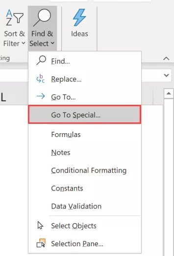
Go to the Editing group and select “Find and Select.”
Select “Go To Special” by clicking. The Go-To Special dialogue box will then be shown.
Choose “Blanks” from the Go-To Special dialogue box.
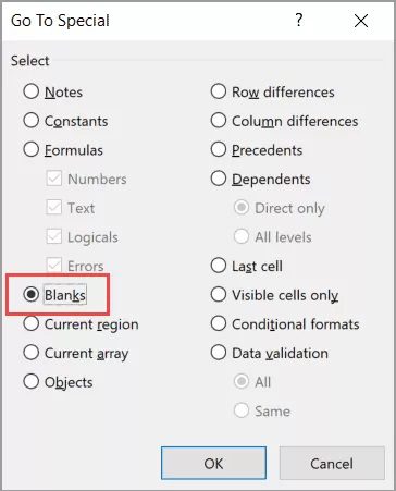
Input OK.

The aforementioned procedures would only pick the blank cells that had previously been a part of the merged cells but had now become empty.

Now use the actions listed below to paste the initial value into these empty cells.

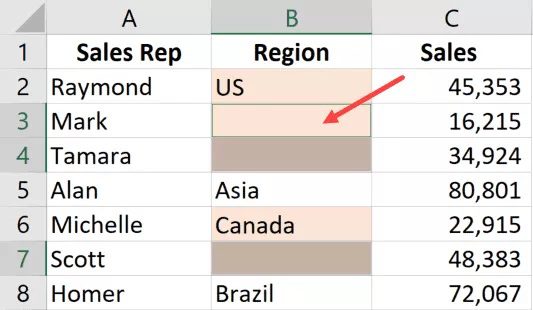
One blank cell has been chosen, and it is highlighted since it is the active cell.

To equalize, use the equals (=) key. the active cell will now display the equal symbol.

Use the up arrow to move up. The cell reference of the cell immediately above the active cell will be picked up by this.

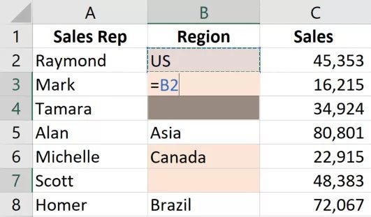
Press the enter key while maintaining control. The identical formula will be entered in each of these chosen empty cells by this (in such a way that every blank cell would refer to the cell above it and pick the value from there)

You will now notice that every blank cell still has the same value as it had previously.