Skip to content
 Square Root Calculation in Excel (Using Easy Formulas)
It’s remarkable how many different options Excel offers to do the same task. There are, after all, a tonne of fantastic features and functions.
Calculating the square root in Excel is an extremely easy yet frequently required activity.
And as I mentioned, there are several methods to accomplish it in Excel (formulas, VBA, Power Query).
I’ll demonstrate many approaches to computing the square root in Excel in this lesson (and you can choose whatever method you like best).
But first, let me briefly explain what a square root is before I explain how to compute it (feel free to skip to the next section if I get too preachy).
This instruction explains:
1. Describe Square Root. 2. Use the SQRT function to calculate the square root. 3. Square Root Calculation using the Exponential Operator 4. Square Root Calculation using the POWER Function 5. Using Power Query to Find the Square Root 6. how to add the square root symbol () to Excel 6.1 Shortcut to Insert Square Root Symbol 6.2 Place a Formula and the Square Root Symbol there. 6.3 Square Root Symbol Insertion through Custom Number Format Modification
1. Describe Square Root.
A value (let’s say Y) is obtained by multiplying a number (let’s say X) by itself.
Here, X is equal to Y’s square root.
For instance, 10 times 10 equals 100.
In this case, 10 is equal to 100 squared.
I’m done now! It’s easy. But calculating it is not so easy.
For instance, if I asked you to mentally calculate the square root of 50, I’m confident you couldn’t do it (unless you were a math prodigy).
If you’re interested in knowing more, you can find a comprehensive page on it here on Wikipedia.
I’ll demonstrate a few (simple, I promise) ways for you to compute square root in Excel in this lesson.
then let’s get going!
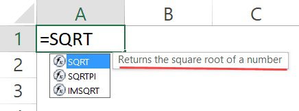
2. Use the SQRT function to calculate the square root.
Yes, Excel has a function specifically designed to provide you with the square root.
The SQRT function returns the square root of a single parameter, which may be a reference to a number or a number itself.
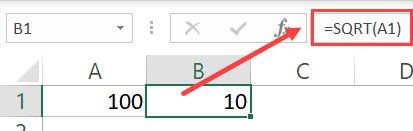
You may use the following formula in Excel to determine the square root of 100:
=SQRT(100)
You can calculate 10 using the method above, which is the square root of 100.
The SQRT function also allows for the usage of cell references, as seen below:
Keep in mind:
Here, a different outcome may be -10, but the method only produces a positive result.
Even if this function excels when given positive integers, it will produce a #NUM error if you supply it with a negative value.
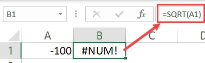
This makes sense because, in mathematics, there is no square root for a negative integer. Even if a number is negative, multiplying it by itself produces a positive result.
However, if you still need to know the square root of a negative number (assumed to be positive), you will first need to change the negative number into a positive one. For instance, you can combine the SQRT function with the ABS function to obtain the square root of -100:
=SQRT(ABS(-100))
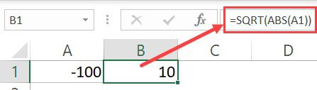
The absolute value is returned by the ABS function, which ignores the negative sign.
Note: Excel has two more square root-related functions:
– SQRTPI
This function calculates the square root of an integer after pi () has been multiplied by it.
– IMSQRT
This function returns the complex number’s square root.
3. Square Root Calculation using the Exponential Operator
Using the exponential operator is another method for calculating the square root in Excel (as well as the cube root and Nth root).
It is simpler to use the SQRT function if all you require is a number’s square root. The exponential operator has the advantage that it may also be used to get the square root, cube root, or nth root.
It may also be used to calculate a number’s square.
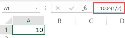
The formula to calculate the square root of 100 is provided below.
=100^(1/2)
and
=100^0.5
Similarly, you may determine a number’s cube root or Nth root.
The calculation for 100’s cube root is shown below.
=100^(1/3)
The calculation for the Nth root of 100 is shown below. (Use any other integer instead of N.)
=100^(1/N)
Notice about brackets:
Make sure to put fractions (like 1/2 or 1/3) in brackets when employing the exponential operator with them. For instance, the outcomes of =100(1/2) and =1001/2 would differ. This is due to the exponential operator being computed first and receiving priority over division. This problem is solved by the use of brackets.
4. Square Root Calculation using the POWER Function
Using the POWER function in Excel is another simple method for finding the square root (or cube root, or Nth root).
The POWER function’s syntax is listed below:
=POWER(number,power)
It needs two justifications:
- the basic quantity (could be any real numbers)
- the exponent or power that this base number is elevated to.
The POWER function can be used to determine a number’s roots or powers, such as its square or cube root, in contrast to the SQRT function.
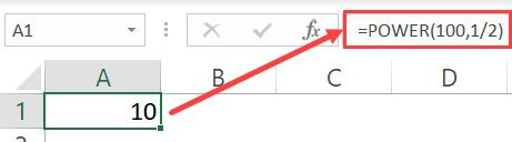
The Excel formula to calculate the square root of 100 is provided below:
=POWER(100,1/2)
or
=POWER(100,.5)
If you need the cube root, use the following formula:
=POWER(100,1/3)
Similarly, you may apply the same technique with the appropriate second input to get the square of a number.
=POWER(100,2)
5. Using Power Query to Find the Square Root
While the aforementioned formulae are rapid, if you work with a lot of data and need to perform this task frequently, you may also take into account utilizing Power Query.
This approach is better suited when you need to get the square root of values in a column over a huge dataset and you receive a fresh dataset every day, week, month, or quarter. Using Power Query will reduce effort since all you have to do is enter in the new data, reload the query, and you’ll get the answer.
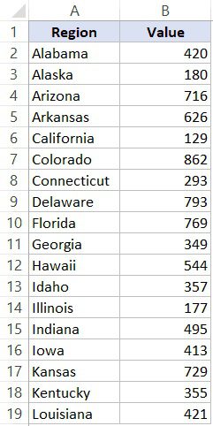
For this demonstration, I’ll use the straightforward dataset depicted below, where I need to square the numbers in column B.
The steps to calculate square root in Excel using Power Query are as follows:
- Choose any cell in the table.
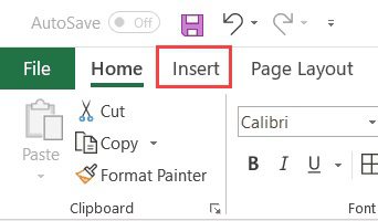
- choose the Insert tab.
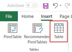
- In the Tables group, select the Table icon. The Create Table dialogue box will then be shown.
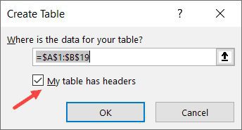
- Check the range and the “My table contains headers” checkbox. Select OK. This will create an Excel Table from the tabular data.
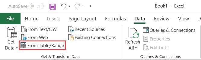
- Go to the Data tab.
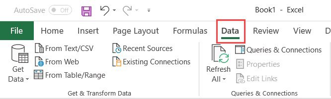
- Select the “From Table/Range” option under the Get & Transform section. The Power Query editor will open.
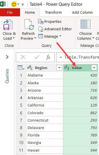
- Click the column header in the Query Editor.
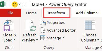
- Select the Transform button.
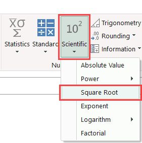
- Select the scientific option from the Number category by clicking it.
- Toggle to Square root. You would receive the square roots of the original numbers along with an immediate update to the values in the chosen column.
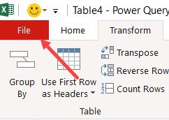
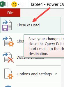
- Go to the File tab.
- Then select Load and Close.
In the Excel workbook, the aforementioned procedures would generate a new worksheet and insert the table from the Power Query. The data from the old table’s square roots will be included in this new table.
If any of the cells contain negative values, a #NUM error will appear in the resultant table.
The wonderful advantage of Power Query is that can now easily refresh and obtain even thought new data, even though their aa a few steps required in making this to work with Power Query.
For instance, if new data becomes available the t month, all you have to do is copy it and paste it into the table we generated in Step 4, then go to any cell in the table you obtained from Power Query, right-click, and select “Refresh.”
As a result, even though it requires a few clicks to complete this the first time, once configured, you may simply change new data by performing a simple refresh.
In addition to the square root, the Power function in Power Query also allows you to obtain the cube root or Nth root (or to get the square or cube of the numbers).
6. How to add the square root symbol (√) to Excel
Despite being somewhat off-topic, I figured I’d also share with you how to enter the square root symbol in Excel.
When displaying value with the square root symbol and its square root next to each other, this might be helpful. as seen below.
Additionally, there are a few ways to insert the square root symbol in Excel, just as there are several formulae available for computing the square root value.
6.1 Shortcut to Insert Square Root Symbol
Here is the keyboard shortcut for entering the square root symbol if you use a numeric keypad:
ALT + 251
Press the 2, 5, and 1 buttons on the numeric keypad while holding down the ALT key. Now, the square root symbol will be added when you leave the keys.
6.2 Place a Formula and the Square Root Symbol there.
Additionally, a formula may be used to find the square root symbol in Excel.
When you want to rapidly apply the square root symbol to all of the values in a column, this might be beneficial.
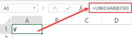
Use the following formula to obtain the square root symbol:
=UNICHAR(8730)
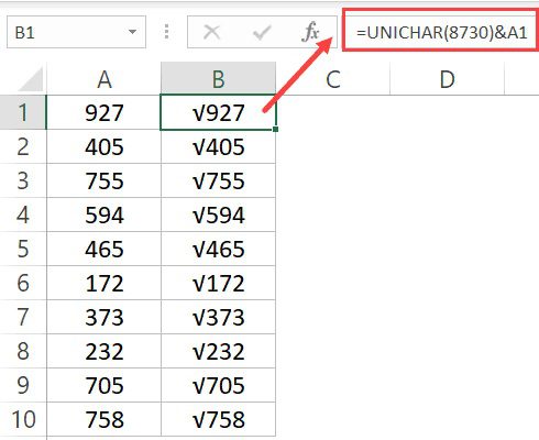
This is a formula, thus you may also use it in conjunction with cell references or other formulae. You may use the following formula, for instance, if you have a column of values and you want to add the square root symbol to each of these values:
=UNICHAR(8730)&A1
Note: If you only need the square root symbol a few times, use the keyboard shortcut or formula to get it the first time, then copy and paste it.
6.3 Square Root Symbol Insertion through Custom Number Format Modification
The third method is to modify the formatting of the cell such that the square root symbol appears anytime you type anything into the cell.
The procedures to modify the cell formatting such that the square root symbol is included automatically are listed below:
- Choose the cells you wish the square root symbol to automatically display in.
- Press the 1 key while maintaining the control key. With this, the Format Cells dialogue box will appear.
- Click on the Custom option in the Category window on the left.
- Fill out the Type box with “General”
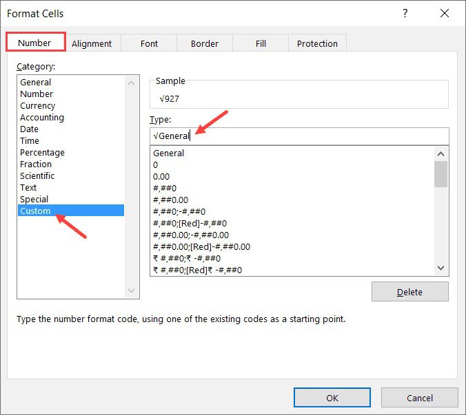
- OK
Once finished, you’ll notice that the square root symbol is immediately applied to all of the selected cells.
Utilizing this approach has the benefit of not altering the cell’s value. It merely modifies the presentation.
This implies that you don’t need to be concerned about the square root symbol interfering when using these numbers in formulae and computations. By picking a cell and checking the formula bar, you may verify this (which shows you the actual value in the cell).