Skip to content
 All About the XLOOKUP Function in Excel (10 Examples)
The XLOOKUP feature in Excel is now available.
I’m sure you’ll like the versatility that the XLOOKUP function offers if you’ve been using VLOOKUP or INDEX/MATCH.
I’ll go over all there is to know about the XLOOKUP function in this lesson, along with a few examples that will show you how to utilize it effectively.
then let’s get going!
This instruction explains: 1. Describe XLOOKUP. 2. Where Can I Find XLOOKUP? 3. Syntax of XLOOKUP Function 4. Examples of XLOOKUP Functions 4.1 Fetch a Lookup Value as an Example 4.2 Example 2: Search for and retrieve a whole record 4.3 Example 3: Using XLOOKUP for a Two-Way Lookup (Horizontal & Vertical Lookup) 4.4 When the Lookup Value is Missing, Example 4 (Error Handling) 4.5 XLOOKUP example 5: Nested (Lookup in Multiple Ranges) 4.6 Find the last matching value in Example 6 4.7 Example 7: Using XLOOKUP to approximate a match (Find Tax Rate) 4.8 Horizontal Lookup Example 8 4.9 Conditional Lookup Example 9 (Using XLOOKUP with Other Formulas) 4.10 Using a wildcard in an XLOOKUP, Example 10 4.11 Find the final value in the column in Example 11 5. If XLOOKUP isn't available, what happens? 6. Backward compatibility for XLOOKUP
1. Describe XLOOKUP.
The VLOOKUP/HLOOKUP function has been updated and is now known as XLOOKUP in Office 365.
It does all of the functions of VLOOKUP plus a lot more.
With the help of the XLOOKUP function, you can rapidly find a value in a dataset (vertically or horizontally) and get the value in the adjacent row or column.
For instance, you can use XLOOKUP to rapidly determine a student’s score using their name if you have the exam results for the students.
Later in this course, when I go in-depth with certain XLOOKUP examples, the value of this method will become even more obvious.
The real concern is, though, how can I get XLOOKUP before I go into the examples?
2. Where Can I Find XLOOKUP?
XLOOKUP is currently only accessible to Office 365 customers.
So you won’t be able to utilize this function if you’re using Excel 2010/2013/2016/2019 or before.
Additionally, I’m not sure whether this will ever be made available for earlier versions (maybe Microsoft can create an add-in the way they did for Power Query). However, as of the right moment, you can only use it if you have Office 365.
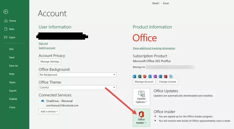
You may access it by going to the File tab and then clicking on Account if you already have Office 365 (Home, Personal, or University version) and don’t have access to it.
You may click to sign up for the Office Insider Program if there is one, and it will be available. You will then have access to the XLOOKUP feature.
I anticipate that all Office 365 versions will shortly support XLOOKUP.
Recall that Excel for the Web and Office 365 for Mac both support XLOOKUP (Excel online)
3. Syntax of XLOOKUP Function
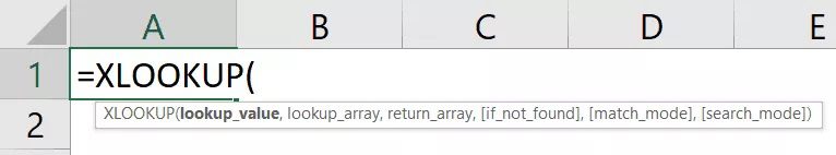
The syntax of the XLOOKUP function is as follows:
=XLOOKUP(lookup_value, lookup_array, return_array, [if_not_found], [match_mode], [search_mode])
You’ll see that the syntax is fairly similar to VLOOKUP, with some fantastic extra capabilities of course.
If the syntax and reasoning seem a little over the top, don’t worry. Later in this course, I address them with some simple XLOOKUP examples to make everything very apparent.
The XLOOKUP method accepts 6 arguments—3 required and 3 optional—as follows:
search value – the worth that you’re seeking
search array- the array you are searching for the lookup value in
returns an array- the array where you wish to get and output the value (corresponding to the position where the lookup value is found)
If not found- the value that will be returned if the lookup value cannot be located. If you omit this option, a #N/A error will be shown.
Matching mode – You may choose the kind of match you want here:
0 – Exact match: The lookup value and the value in the lookup array should match perfectly. The default choice is this.
-1 – searches for the exact match, but if one is discovered, returns the next smaller item or value.
1 – Finds the closest match first, but if one is found, returns the next bigger thing or value.
2_ utilizing wildcards (* or ) to perform partial matching
In search mode- Here, you tell the XLOOKUP function how to look up data in the lookup array.
1 – The function searches for the lookup value in the lookup array starting at the top (first item) and moving down (last item) in this default setting.
-1 – Search from bottom to top. helpful for looking up the last matched value in a lookup _array
2 – Carry out a binary search when the information must be arranged in ascending order. This might produce inaccurate results if it is not sorted.
-2 – when the data must be sorted in descending order, do a binary search. This might produce inaccurate results if it is not sorted.
4. Examples of XLOOKUP Functions
Let’s move on to the intriguing part, which is some real-world XLOOKUP instances.
With the aid of these examples, you will be better able to comprehend how XLOOKUP operates, how it differs from VLOOKUP and INDEX/MATCH, as well as some of its advantages and disadvantages.
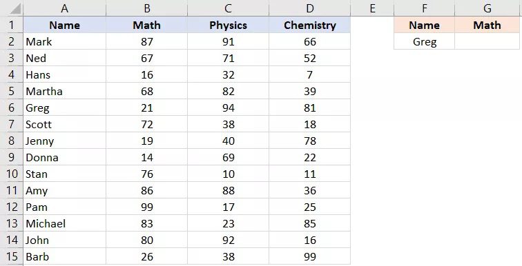
4.1 Fetch a Lookup Value as an Example
Assume you wish to retrieve Greg’s math score from the dataset below (the lookup value).
The formula for doing this is as follows:
=XLOOKUP(F2,A2:A15,B2:B15)
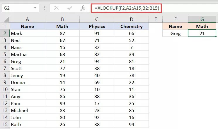
I have just used the necessary inputs in the formula above, which searches for the name (from top to bottom), finds an exact match, and then returns the matching value from B2 to B15.
The way the LOOKUP and VLOOKUP functions handle lookup arrays is one clear distinction between them. In VLOOKUP, you first give the column number from which you wish to get the result after having the whole array with the lookup value in the leftmost column. On the other hand, XLOOKUP lets you select the lookup array and return the array independently.
You may now look to the left as a direct result of having the lookup array and return array as independent inputs. The only value that could be looked for and found using VLOOKUP is to the right. XLOOKUP, however, removes that restriction.
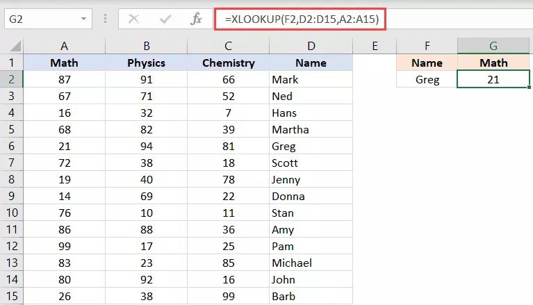
Here’s an illustration. The name is on the right and the return range is on the left in the dataset I’m using.
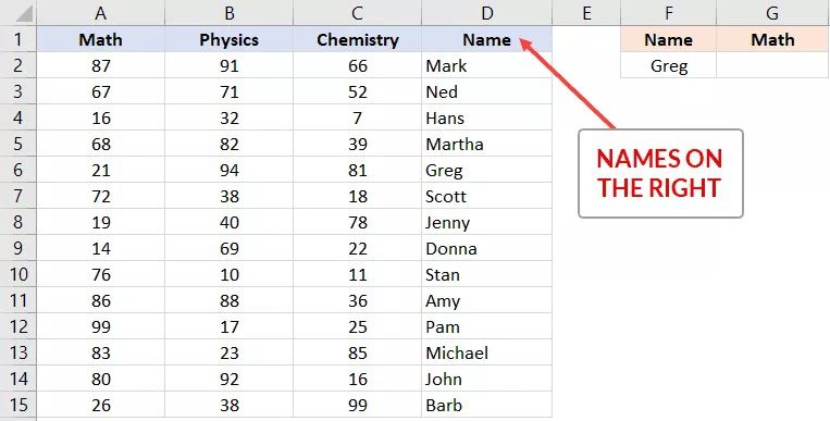
I can use the formula listed below to get Greg’s math grade by looking to the left of the lookup value.
=XLOOKUP(F2,D2:D15,A2:A15)
Another significant problem that is resolved by XLOOKUP is that the generated data will remain accurate even if you insert a new column or rearrange existing ones. In these circumstances, VLOOKUP would probably malfunction or produce an inaccurate result since the column index value is frequently hard-coded.
4.2 Example 2: Search for and retrieve a whole record
Let’s use identical data as an illustration.
I don’t want to just retrieve Greg’s math grade in this situation. I aim to achieve the required grades across the board.
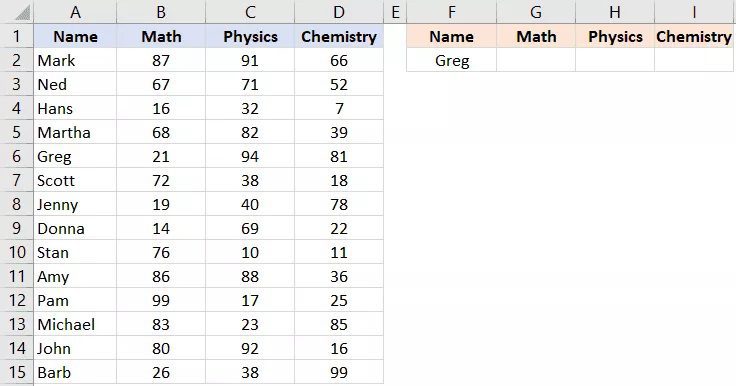
In this situation, I may use the formula below:
=XLOOKUP(F2,A2:A15,B2:D15)
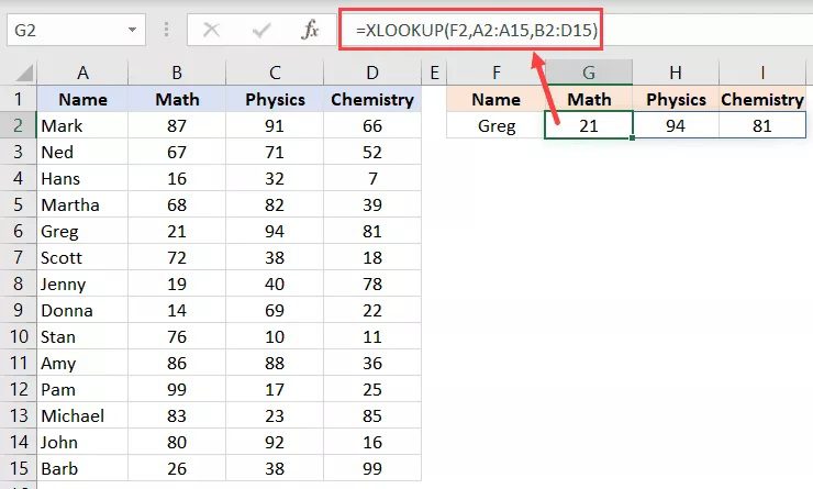
The formula above uses a return array range larger than a single column (B2:D15). Therefore, the formula returns the complete row from the return array when the lookup value is located in A2:A15.
Additionally, only the cells that are a part of the array and were filled automatically cannot be deleted. You cannot remove H2 or I2 in this case. Nothing would happen if you tried. The formula in the formula bar would be greyed out if you selected these cells (indicating that it can not be changed)
The formula may be removed from cell G2 (where it was initially inserted), which will also remove the complete result.
This is a helpful improvement since previously when using VLOOKUP, you had to provide the column number individually for each formula.
4.3 Example 3: Using XLOOKUP for a Two-Way Lookup (Horizontal & Vertical Lookup)
Here is a dataset where I want to know Greg’s math grade (the subject in cell G2).

Using a two-way lookup, I can find the name in column A and the topic name in row 1 to do this. The advantage of this two-way query is that the outcome may be determined regardless of the subject name or student name. This two-way XLOOKUP formula would still function and get the right results if I changed the topic name to Chemistry.
The equation that will carry out the two-way lookup and provide the desired outcome is shown below:
=XLOOKUP(G1,B1:D1,XLOOKUP(F2,A2:A15,B2:D15))
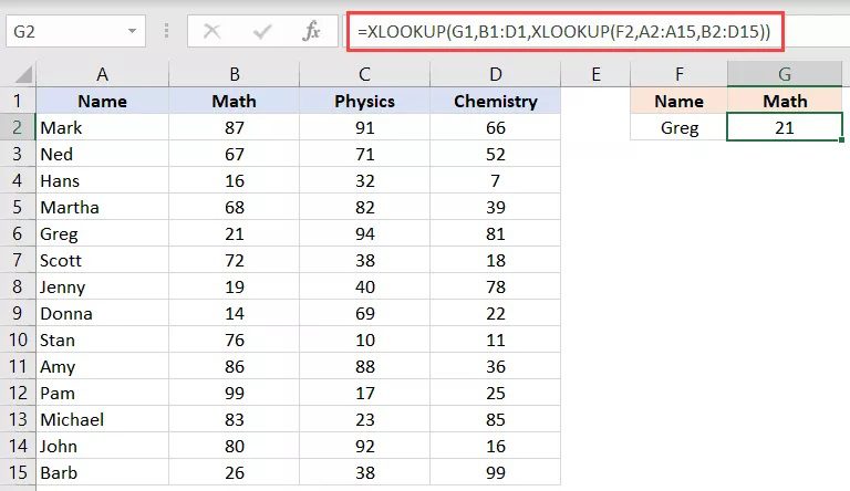
Nested XLOOKUP is used in this calculation, and I first use it to retrieve all the student’s grades in cell F2.
Thus, the output of XLOOKUP(F2, A2:A15, B2:D15 ) is 21,94,81, which in this example represents an array of the grades Greg received.
This is then utilized once more as the return array in the outer XLOOKUP expression. I search for the subject name (which is in cell G1) using the outer XLOOKUP formula, and the lookup array is B1:D1.
This outer XLOOKUP formula retrieves the first value from the return array, which in this case is 21,94,81 if the topic name is Math.
This accomplishes the same thing that the INDEX and MATCH combination did up until this point.
4.4 When the Lookup Value is Missing, Example 4 (Error Handling)
The XLOOKUP formula has been updated to provide error handling.
The [if not found] option in the XLOOKUP function’s fourth argument allows you to define what you wish to happen if the lookup is unsuccessful.
Consider the following dataset, where you wish to return “Did not appear” if the name cannot be identified and the Math score in the event of a match.
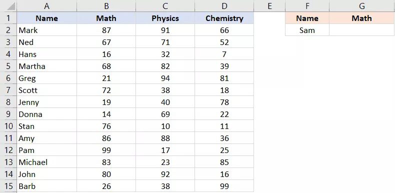
This may be accomplished using the formula below:
=XLOOKUP(F2,A2:A15,B2:B15,"Did not appear")
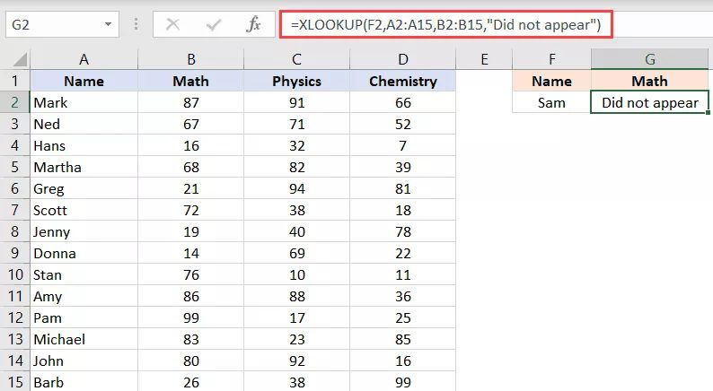
In this instance, if there is no match, I have hard-coded what I wish to get. A cell reference can also be used to refer to a cell or a formula.
4.5 XLOOKUP example 5: Nested (Lookup in Multiple Ranges)
The [if not found] argument’s brilliance is that it enables the usage of nested XLOOKUP formulas.
Assume, for instance, that you have the two independent lists displayed below. Although I have these two tables on one sheet, you could have them on different sheets or even in a workbook.
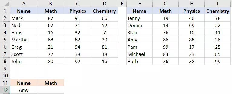
The nested XLOOKUP formula is shown below. It will search both tables for the name and return the relevant value from the chosen column.
=XLOOKUP(A12,A2:A8,B2:B8,XLOOKUP(A12,F2:F8,G2:G8))
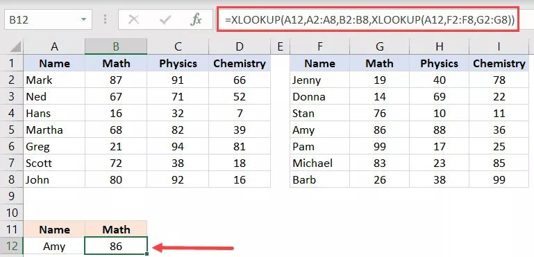
I utilized another XLOOKUP formula in the formula above using the [if not found] parameter. This enables you to incorporate a second XLOOKUP into the calculation and scan two tables simultaneously.
How many nested XLOOKUPs are allowed in a formula? I’m not sure. I persisted till 10 p.m. and it finally worked.
4.6 Find the last matching value in Example 6
A lot of people wanted this one, and XLOOKUP made it feasible. The final matching value in a range no longer has to be obtained by using complicated methods.
Assume you have the dataset depicted below and wish to determine the date of the most recent hire in each department.
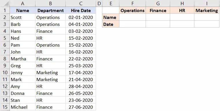
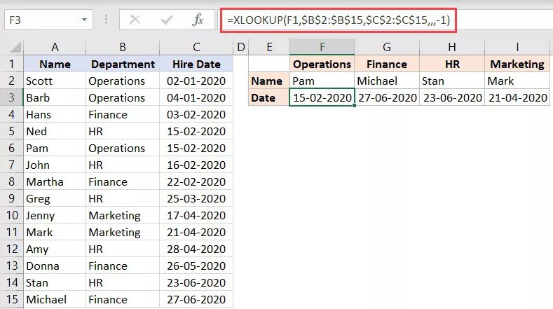
The formula below will get the most recent value for each department and display the name of the most recent hire:
=XLOOKUP(F1,$B$2:$B$15,$A$2:$A$15,,,-1)
Additionally, the formula below will provide the most recent recruitment date for each department:
=XLOOKUP(F1,$B$2:$B$15,$C$2:$C$15,,,-1)
A straightforward formula is used to indicate the lookup direction (first to last or last to first), which is an intrinsic feature of XLOOKUP. VLOOKUP and INDEX/MATCH always look at vertical data from top to bottom, while XLOOKUP also allows you to define the direction from bottom to top.
4.7 Example 7: Using XLOOKUP to approximate a match (Find Tax Rate)
The addition of four match modes to XLOOKUP is another noteworthy development (VLOOKUP has 2 and MATCH has 3).
The lookup value should be matched using one of the four parameters, which you can specify:
- 0 – Exact match: The lookup value and the value in the lookup array should match perfectly. The default choice is this.
- -1 – Finds the closest match first, but if one is found, returns the next smaller item or value.
- 1 – searches for the identical match, but if it is discovered, returns the following bigger item or value.
- 2 – Using wildcards (* or ) to do partial matching
Best of all, you don’t have to worry about whether your data is sorted in ascending or descending order. XLOOKUP will take care of the problem even if the data is not sorted.
The dataset I’m working with below contains information on each person’s commission, which must be computed using the right-hand table.

The equation to accomplish this is given below:
=XLOOKUP(B2,$E$2:$E$6,$F$2:$F$6,0,-1)*B2
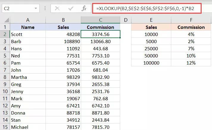
This only searches the lookup table on the right using the sales value as the lookup. Since I used -1 as the fifth input ([match mode]) in this formula, it will first search for an exact match before returning a result that is just below the lookup value.
As I previously stated, you don’t need to be concerned with how your data is organized.
4.8 Horizontal Lookup Example 8
Both vertical and horizontal lookups are possible with XLOOKUP.
I want to retrieve the score for the name in column B7 in the dataset below, which contains student names and their scores in rows.
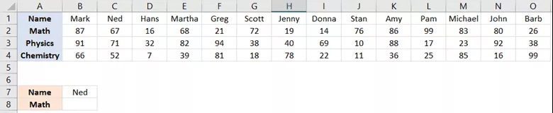
This may be accomplished using the formula below:
=XLOOKUP(B7,B1:O1,B2:O2)
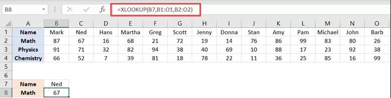
This is nothing more than a straightforward horizontal search, identical to what we saw in Example 1.
With the use of XLOOKUP, all the vertical lookup examples I provide may also be performed horizontally (farewell to VLOOKUP and HLOOKUP).
4.9 Conditional Lookup Example 9 (Using XLOOKUP with Other Formulas)
This example, which is a little more sophisticated, demonstrates the potential of XLOOKUP when doing intricate lookups.
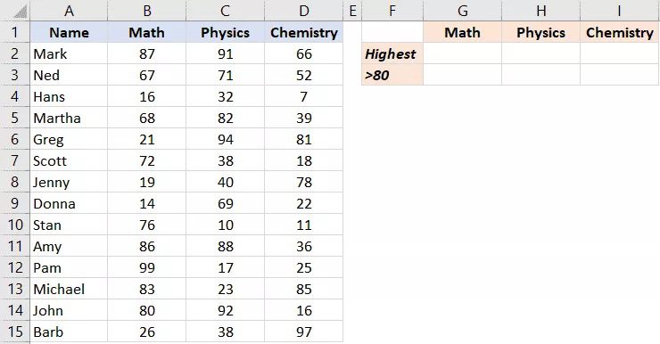
I have a data file with student names and scores below, and I’m interested in knowing who had the highest score in each topic as well as how many students received scores of 80 or above in each subject.
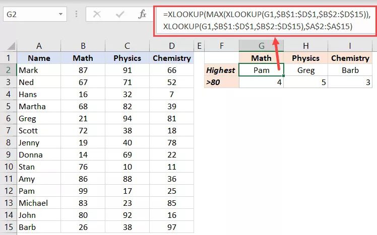
The equation that will identify the student who received the best score in each topic is as follows:
=XLOOKUP(MAX(XLOOKUP(G1,$B$1:$D$1,$B$2:$D$15)),XLOOKUP(G1,$B$1:$D$1,$B$2:$D$15),$A$2:$A$15)
I used XLOOKUP to initially obtain all the marks for the relevant topic as it can be used to retrieve a complete array.
For instance, using XLOOKUP(G1,$B$1:$D$1,$B$2:$D$15) for math returns all of the results. The highest score within this range can then be discovered using the MAX function.
The array given by XLOOKUP(G1,$B) would represent my search range, and this highest score would serve as my lookup value.
$1:$D$1,$B$2:$D$15)
I include this in another XLOOKUP calculation to retrieve the name of the student with the highest grade.
Use the following calculation to determine how many students received a score of 80 or higher:
=COUNTIF(XLOOKUP(G1,$B$1:$D$1,$B$2:$D$15),">80")
The XLOOKUP formula is all that is used in this case to obtain a range of all the values for the specified subject. To determine how many scores are more than 80, it is then wrapped in the COUNTIF function.
4.10 Using a wildcard in an XLOOKUP, Example 10
With XLOOKUP, you can utilize wildcard characters in the same way that you can with VLOOKUP and MATCH.
However, there is a distinction.
You must indicate that you’re utilizing wildcard characters in XLOOKUP (in the fifth argument). This must be specified else XLOOKUP will return an error.
I have a dataset with firm names and their market capitalization down below.
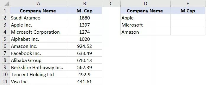
I want to get the market capitalization of a certain firm by looking up its name in column D and the table to the left. Additionally, I will need to utilize wildcard characters because the names in Column D are not exact matches.
The equation to accomplish this is given below:
=XLOOKUP("*"&D2&"*",$A$2:$A$11,$B$2:$B$11,,2) 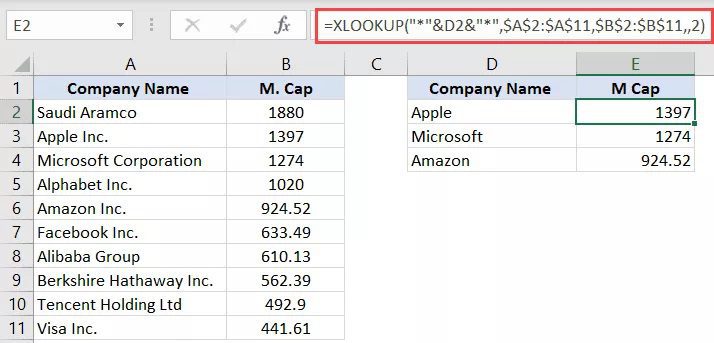
I used the asterisk (*) wildcard character before D2 in the calculation above (it needs to be within double quotes and joined with D2 using ampersand).
This instructs the formula to search all the cells for the word in cell D2 (Apple), and if it finds it, to treat it as an exact match. Regardless of the number and kind of letters that come before and after the content in cell D2.
Additionally, the fifth parameter has been adjusted to 2 to ensure that XLOOKUP allows wildcard characters (wildcard character match).
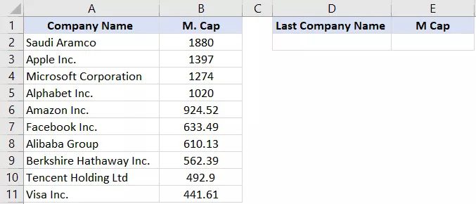
4.11 Find the final value in the column in Example 11
Since XLOOKUP enables bottom-to-top searching, it is simple to locate the final item in a list and retrieve the matching value from a column.
Assume you have the dataset depicted below and are interested in learning about the last firm and its market capitalization.
The last company’s name may be determined using the formula below:
=XLOOKUP("*",A2:A11,A2:A11,,2,-1) The market cap of the final firm on the list may be calculated using the method below:
=XLOOKUP("*",A2:A11,B2:B11,,2,-1) 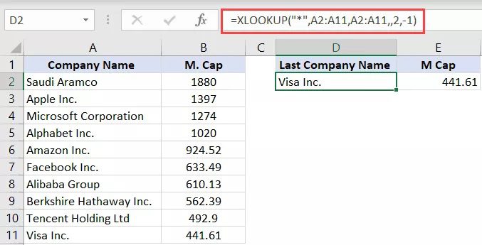
The same wildcard characters are used in these calculations. The lookup value in these is an asterisk (*), which indicates that the first cell it sees will be treated as an exact match (as an asterisk could be any character and any number of characters).
The final value in the list will be returned since the direction (for the vertically ordered data) is from bottom to top.
And to get the market capitalization of the final name in the list, the second calculation employs a different return range.
5. If XLOOKUP isn’t available, what happens?
One approach to obtain XLOOKUP is to upgrade to Office 365 as it is probable that only Office 365 customers will have access to it.
You already have access to XLOOKUP if you already have Office 365 Home, Personal, or University edition. Simply enrolling in the Office Insider program will do.
I’m sure XLOOKUP and other wonderful features (such dynamic as arrays, and formulae like SORT and FILTER), would soon be available if you have additional Office 365 subscriptions (like Enterprise).
If you’re still using Excel 2010/2013/2016/2019, you’ll still need to utilize VLOOKUP, HLOOKUP, and the INDEX/MATCH combination to get the most out of lookup formulae because XLOOKUP isn’t available.
6. Backward compatibility for XLOOKUP
You must be careful about this since XLOOKUP is NOT backward compatible.
As a result, a file created using the XLOOKUP formula will display errors when opened in a version that does not support XLOOKUP.
Although it will probably take a few years before XLOOKUP is widely used, I think it will eventually become the standard lookup formula since it is a significant step in the right direction. After all, I continue to encounter users using Excel 2003.
These 11 XLOOKUP examples will speed up your search and reference work while also making it simple to use.