Ms Excel VBA Teach You A simple chart in Excel can say more than a sheet full of numbers. As you will see, creating
charts are extremely easy.
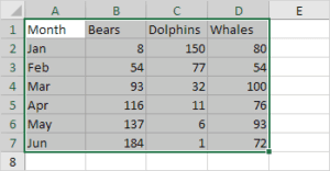
1: Select the range A1:D7
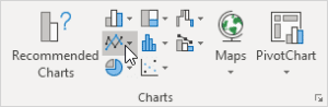
2. On the Insert tab
In the Charts group, Click the Line symbol.
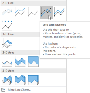
3. Click Line with Markers!
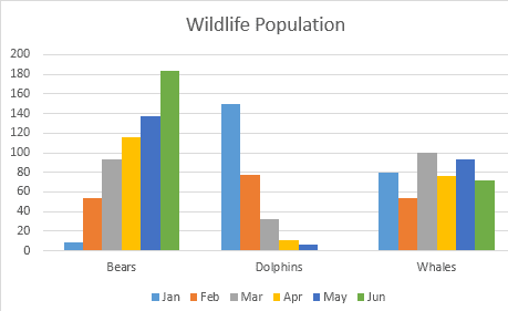
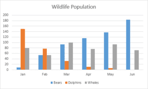
4. Results_:
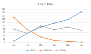
Note: Enter a title by clicking on the Chart Title.
For example, a Wildlife Population.
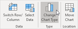
Change Chart Type
You can easily change to a different type of chart at any time when you want!
1. Select the chart.
2. On the Chart Design tab, in the Type Of group, click Change Chart Type
3. On the left side, click Column.
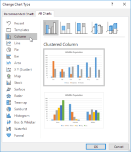
4. Hit OK.
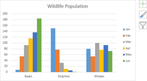
5. Here is the Result
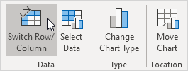
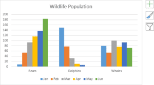
Switch Row/ Column
Still, execute the following way, If you want to display the creatures( rather than the months) on the vertical axis.
1. Select the chart.
2. On the Chart Design tab, in the Data group, click Switch Row/Column.
3. Result:
Legend Position
To move the legend to the right side of the chart, execute the following route.
1. choose the chart.
2. Click the push button on the exact side of the chart, Choose the arrow next to Legend and click Right.
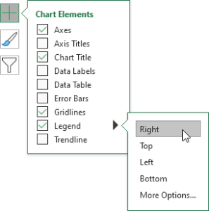
3. Result:
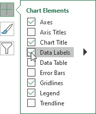
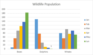
Data Markers
You can use data markers to concentrate your albums‘ absorption on a single data series or data point.
1. Choose the chart.
2. commune a green bar to select the Jun data series.
3. Hold down CTRL and apply your arrow keys to select the population of Dolphins in June( bitsy green bar).
4. Click the push button on the exact side of the chart and click the check box next to Data Labels.
Here is the Result:
Learn more about the Charts with Us!
Learn Complete Microsoft Excel Tutorial