Examples and a video explaining the Excel filter function
Office 365 has some fantastic features, like XLOOKUP, SORT, and FILTER.
Before Office 365, we relied only on Excel’s built-in filter, the Advanced filter at most, or complicated SUMPRODUCT formulae to filter data in Excel. It was often a difficult workaround if you needed to filter a specific portion of a dataset (something I have covered here).
However, it’s now incredibly simple to quickly filter a portion of the dataset based on criteria thanks to the new FILTER function.
And I’ll demonstrate how fantastic the new FILTER function is and some practical uses for it in this lesson.
But first, let’s quickly review the FILTER function’s syntax before moving on to the examples.
If you want access to all of the new capabilities in Excel, you may upgrade to Office 365 (join the insider program to do so).
This instruction explains:

1. Syntax for the Excel filter function
2. Example 1: Data Filtering Using a Single Criteria (Region)
3. Example 2: Data Filtering Using a Single Criteria (More Than or Less Than)
4. Example 3: Multiple-criteria data filtering (AND)
5. Example 4: Multiple-criteria data filtering (OR)
6. Example 5: Getting Above/Below Average Records by Filtering Data
7. Example 6: Strictly Filtering Records with Even Numbers (Or ODD Number Records)
8. Example 7: Using a Formula to Sort the Filtered Data
1. Syntax for the Excel filter function
The FILTER function’s syntax is listed below:
=FILTER(array,include,[if_empty])
array:
This is the set of cells where the data that you wish to filter from is located.
include –
It is in this situation that the function is instructed to filter certain entries.
[if_empty] –
You can define what to return using this optional parameter if the FILTER function returns no results. When not supplied, it defaults to returning the #CALC! error.
Let’s look at some incredible Filter function examples and what it can achieve now that it used to be pretty difficult to perform before.
2. Example 1: Data Filtering Using a Single Criteria (Region)
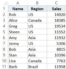
Let’s say you want to filter all the records for those that are from the US exclusively and you have the dataset as shown below.
The FILTER formula to accomplish this is listed below:
=FILTER($A$2:$C$11,$B$2:$B$11="US")
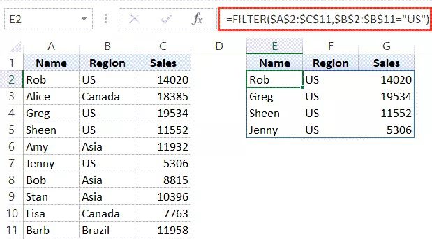
The dataset is used as an array in the calculation above, and the criterion is $B$2:$B$11=”US.”
The FILTER function would examine each cell in column B (the column that contains the region) as a result of this condition, and only records that satisfied this requirement would be filtered.
The original data and the filtered data are both on the same page in this example, but you may alternatively have them on other sheets or even in different workbooks.
A dynamic array is a result that the filter function returns (which means that instead of returning one value, it returns an array that spills to other cells).
You need to have a location where the outcome would lead to being empty for this to work. The function will give you the #SPILL error if any of the cells in this area (E2 to G5 in this example) already have content in them.
Additionally, as this is a dynamic array, you cannot alter a specific portion of the outcome. Cell E2 or the whole range containing the result can be deleted (where the formula was entered). Both of these would eliminate the whole array that was produced. However, you cannot alter a single cell (or delete it).
Although I have hard-coded the region value in the calculation above, you may also store it in a cell and then reference that cell.
For instance, in the example below, cell I2 has the region value, which is subsequently used as a reference in the formula:
=FILTER($A$2:$C$11,$B$2:$B$11=I1)
The filter may now be changed by simply changing the region value in cell I2 and the formula has become even more helpful.
You may also have a drop-down in cell I2 where you can choose something and the filtered data will be updated right away.
3. Example 2: Data Filtering Using a Single Criteria (More Than or Less Than)
Additionally, you may extract all the records that are greater or lesser than a certain value by using comparison operators within the filter function.
Consider the following dataset as an example. Suppose you wish to filter out all the entries where the sales value exceeds 10,000.

Using the formula below, you can:
=FILTER($A$2:$C$11,($C$2:$C$11>10000))

The full dataset is referred to by the array argument in this example, and the condition is ($C$2:$C$11>10000).
The value in Column C is checked by the formula against each entry. The value is filtered if it exceeds 10,000; else, it is ignored.
If you want to obtain every record that is fewer than 10,000, use the formula below:
=FILTER($A$2:$C$11,($C$2:$C$11<10000))
The FILTER formula also offers additional creative possibilities. For instance, you can use the following formula to filter the top three records based on sales value:
=FILTER($A$2:$C$11,($C$2:$C$11>=LARGE(C2:C11,3)))
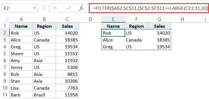
The third biggest value in the dataset is obtained using the LARGE function in the formula above. The FILTER function criterion uses this value to find all the entries whose sales value is greater than or equal to the third-largest value.
4. Example 3: Multiple-criteria data filtering (AND)
Assume you have the dataset below and wish to filter out all the US entries where the selling amount is greater than 10,000.
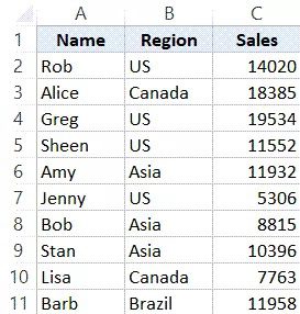
This is an AND condition, so you have to be sure of two things: that the region is the US and that there have been more than 10,000 sales. The results shouldn’t be filtered if only one requirement is satisfied.
The FILTER formula is listed below, and it will filter records with sales of more than 10,000 with the US as the region:
=FILTER($A$2:$C$11,($B$2:$B$11="US")*($C$2:$C$11>10000))
Please take note that the requirement is ($B$2:$B$11=”US”)*($C$2:$C$11>10000).
I have used the multiplication operator to combine these two conditions since I am employing two conditions and I need both of them to be true. This produces an array of 0s and 1s, with a 1 only appearing when both requirements are satisfied.
The function would return the #CALC! error if no records met the requirements.
Additionally, you may use the following formula if you want to return something meaningful rather than the error:
=FILTER($A$2:$C$11,($B$2:$B$11="USA")*($C$2:$C$11>10000),"Nothing Found")
The final argument, in this case, is “Not Found,” which is used when no entries are discovered that satisfy the criteria.
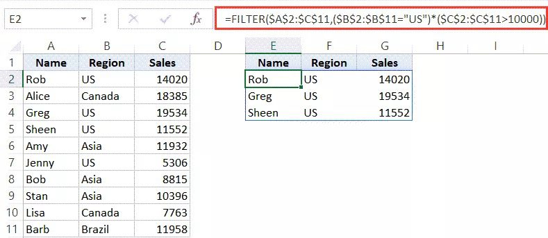
5. Example 4: Multiple-criteria data filtering (OR)
Additionally, you may change the FILTER function’s “include” parameter to check for an OR criterion (where any one of the given conditions can be true).
Consider the following dataset as an example. You might wish to filter the entries where either the US or Canada is listed as the nation.

The equation to accomplish this is given below:
=FILTER($A$2:$C$11,($B$2:$B$11="US")+($B$2:$B$11="Canada"))
Note:
that I simply combined the two criteria by using the addition operator in the calculation above. Since each of these criteria yields an array of TRUEs and FALSEs, I can combine them to get an array that is TRUE if any one of the requirements is satisfied.
Another example would be to filter all records where either the nation is the United States or the selling value is greater than $10,000.
This may be accomplished using the formula below:
=FILTER($A$2:$C$11,($B$2:$B$11="US")+(C2:C11>10000))
Note: In a FILTER function, use the multiplication operator (*) for AND criteria and the addition operator (+) for OR criteria.
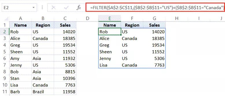
6. Example 5: Getting Above/Below Average Records by Filtering Data
To filter and extract records where the value is above or below the average, utilize formulae within the FILTER function.
Consider the following dataset as an example. Suppose you want to filter out all the records where the selling value is higher than average.

Utilizing the following formula, you may achieve that:
=FILTER($A$2:$C$11,C2:C11>AVERAGE(C2:C11))
The following formula can be used for below-average:
=FILTER($A$2:$C$11,C2:C11<AVERAGE(C2:C11))
7. Example 6: Strictly Filtering Records with Even Numbers (Or ODD Number Records)
The FILTER function allows you to easily filter and retrieve all the data from rows with an even or odd number of characters.
To do this, use the FILTER function to verify the row number and only filter out row numbers that match the requirements.
Let’s say you have the dataset depicted below, and I only want to extract records with even numbers from it.

The equation to accomplish this is given below:
=FILTER($A$2:$C$11,MOD(ROW(A2:A11)-1,2)=0)
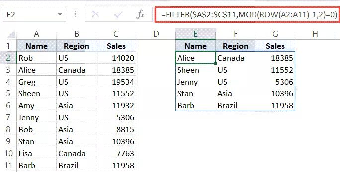
The MOD function is used in the formula aforementioned to determine each record’s row number (which is given by the ROW function).
When the row number is even, the formula MOD(ROW(A2:A11)-1,2)=0 yields TRUE; when it is odd, it returns FALSE. As the initial record is in the second row, the row number is adjusted to take the second row into account and I have deducted 1 from the ROW(A2:A11) portion to reflect this.
The formula below may be used to filter all the records with odd numbers.
=FILTER($A$2:$C$11,MOD(ROW(A2:A11)-1,2)=1)
8. Example 7: Using a Formula to Sort the Filtered Data
We can accomplish much more when we combine the FILTER function with additional functions.
For instance, you may combine the SORT function with the FILTER function to obtain the result of a filtered dataset that has already been sorted.
Assume you want to filter all the entries where the sales value is more than 10,000 in a dataset like the one below. To ensure that the data is sorted according to the sales value, use the SORT function together with the function.

This may be accomplished using the formula below:
=SORT(FILTER($A$2:$C$11,($C$2:$C$11>10000)),3,-1)
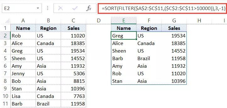
To get the data where the sale value in column C is more than 10,000, the aforementioned code uses the FILTER function. The SORT function then sorts this data according to the sales value using the array given by the FILTER function.
The third column should be used as the sorting criteria in the second parameter of the SORT function, which is 3. The fourth option, -1, causes the data to be sorted in reverse chronological order.
These are the seven examples of how to utilize Excel’s FILTER function.