Skip to content
 Excel: Remove Left Characters (Easy Formulas):
For many Excel users, cleaning text data is frequently the most time-consuming operation.
Unless you’re one of the select few, you’ll probably receive your data in a format that requires some cleaning.
When you receive a dataset and need to eliminate certain characters from the left for this dataset, that would be one typical use case for this.
You may have a certain amount of characters to delete from the left, or they may come before a particular letter or string.
In this article, I’ll walk you through a few straightforward examples of taking off the necessary number of characters from the left side of a text string.
This instruction explains:
1. Getting Rid of the Left Fixed Number of Characters
2. Characters from the Left are Removed Based on the Delimiter (Space, Comma, Dash)
2.1 Applying the Correct Formula
    2.2 Flash Filling
    2.3 How to Use Text to Columns
3 Remove every word to the left of a certain string
4. Eliminate all left-side text (and keep the numbers)
5. Take Off Every Number to the Left
1. Getting Rid of the Left Fixed Number of Characters:
You may use the method demonstrated here to delete a certain number of characters from the left of the string in each cell if you obtain a dataset that is consistent and follows the same pattern.
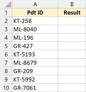
I want to extract only the numbers from the product in the dataset below, which are composed of a two-letter code and a number (which means that I want to remove the first three characters from each cell).

The formula to achieve this is as follows:
=RIGHT(A2,LEN(A2)-3)
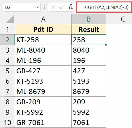
The LEN function is used in the formula above to determine how many characters are present in each cell in column A.
We deduct 3 from the value obtained by the LEN function because we just need to extract the numbers and want to get rid of the first three characters from the string to the left of each cell.
The RIGHT function then uses this value to remove all characters from the left except for the first three.
This approach would only be practical if you always wanted to delete the specified number of characters from the left since the number of characters we want to remove from the left has been hardcoded. The formula above would not work if the data mentioned above were inconsistent and the number of characters preceding the number varied (use the formula next section in such a scenario).
2. Characters from the Left are Removed Based on the Delimiter (Space, Comma, Dash):
Most of the time, it is rare that you will obtain data that is consistent when the number of letters you wish to delete from the left has a constant length.
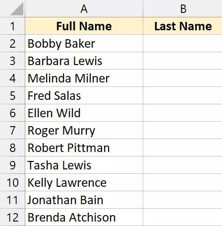
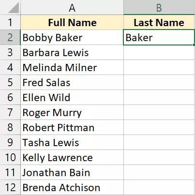
For instance, in the names dataset below, I have the first name to be removed so that I only receive the last name.

Additionally, as you can see, the initial name’s length fluctuates. Thus I am unable to utilize the method described in the preceding part.
In this situation, I still need to rely on a reliable pattern, which would be a space character to separate the first and last names.
If I could delete everything until the space character, I would get the intended outcome.
And there are several methods to achieve this owing to Excel’s fantastic capabilities.
2.1 Applying the Correct Formula:
Let’s look at a formula that will only leave the last name after the space character after removing everything else.
=RIGHT(TRIM(A2),LEN(TRIM(A2))-FIND(" ",TRIM(A2))) 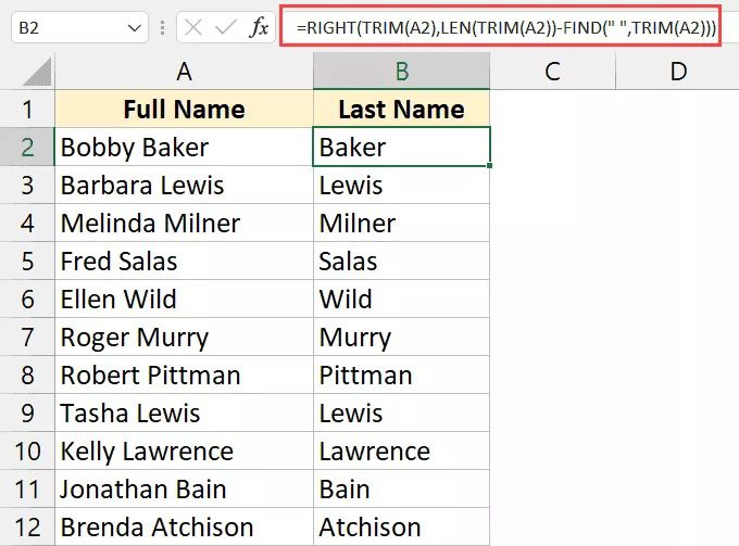
By using the aforementioned technique, you may retrieve the remaining text by removing anything to the left of the space character, including the space character (last name in this example).
Let me briefly go through the operation of this formula.
To start, I located the space character in the cell using the FIND tool.
FIND(” “, TRIM(A2)) would yield 6 in the calculation above since the space character appears in cell A2’s name in the sixth place.
The total number of characters in the cell following the space character was determined by subtracting the value returned by the FIND function from the value obtained using the LEN function.
I’ve used the RIGHT function to extract the rightmost characters now that I know how many characters to take out of the text string.
To ensure that any leading, trailing, or double spaces are handled in the formula above
I utilized the TRIM function.
One major advantage of employing a formula is that, if you modify any of the values in Column A, the results will update immediately.
2.2 Flash Filling:
Using Flash Fill is another extremely rapid method for removing text from the delimiter’s left side.
Flash Fill functions by determining patterns from a few user inputs. In our scenario, I would need to manually type the desired outcome into one or two cells before using Flash Fill to repeat the process in the remaining cells.
Let’s say I have a dataset like the one below and I want to get rid of every character that comes before the space.
The procedures for using flash fill to eliminate characters to the left of a delimiter are as follows:
Insert the anticipated outcome in cell B2 (Baker in this case)
Choose cells B2 through B12 (the range where you want the result)
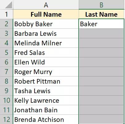
Press the E key while holding down the Control key (or Command + E on a Mac).
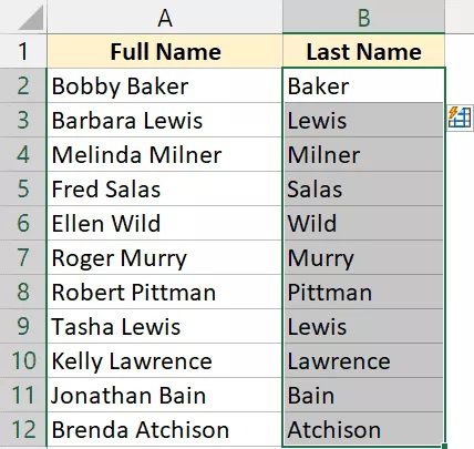
After doing the aforementioned processes, all that would be left after the space character would be the last name.
Keep in mind:
That the keyboard shortcut for Excel's Flash Fill is Control + E (or Command + E on a Mac).
Let me now briefly explain what is going on.
It tries to find the pattern using the result I’ve previously placed in cell B2 when I manually type the anticipated result in cell B2, select all the cells, then use Flash Fill.
In this case, it was able to recognize that I am attempting to delete everything to the left of the final name since I am trying to extract the last name.
As soon as it discovered this pattern, it applied it to every cell in the column.
When utilizing Flash Fill, it is conceivable
that Excel won't always be able to recognize the right pattern. In these circumstances,
you could try inputting the findings many times so that Excel has more information to analyze the trend.
MS EXCEL VBA
3. How to Use Text to Columns:
Using the Text to Columns tool would be another easy approach to eliminate all the characters that come before a delimiter.
Let’s say I want to get rid of anything before the dash from the dataset that is displayed below.
The procedures are as follows:
- Select the data-containing range (A2:A10 in this example)
- Choose the “Data” tab.
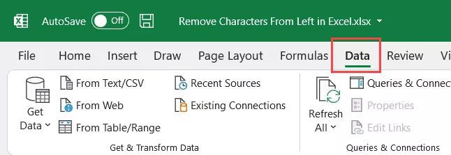
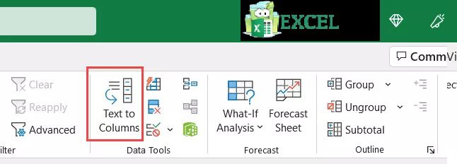
- Go to the Data Tools section and select “Text to Columns.”
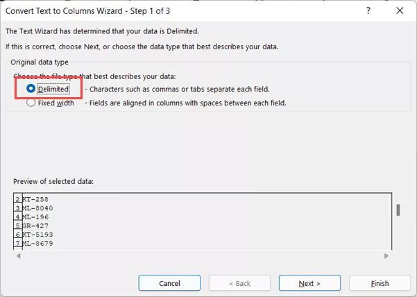
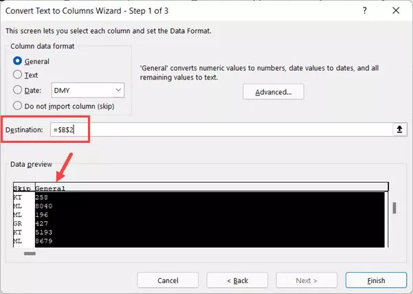
- Step 1 of 3 in the Text to Columns Wizard Ensure that Delimited is chosen.
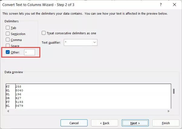
- Step 2 of 3: Enter – in the box next to Other as the Delimiter.
- Choose the “Do Not Import Column (Skip)” option in the third of three steps. Additionally, confirm that the column chosen (in black) in the Data Preview is the one you wish to delete.
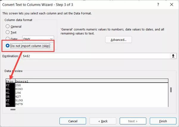
- Step 3 of 3: In Data Preview, choose the desired second column before choosing the last cell (I will go with the already selected B2)
- Select Finish.
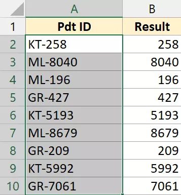
Based on the designated delimiter, the aforementioned stages would divide into distinct columns.
Note:
That I separated the data into distinct columns in this example by using a delimiter.
Text to Columns may also take off a certain number of characters from the left of a text string.
For that, in Step 1 of 3 of the Text to Columns process, select Fixed Length rather than the Delimiter option.
4. Remove every word to the left of a certain string:
In some datasets, you might need to remove all the text that comes before a certain text string.
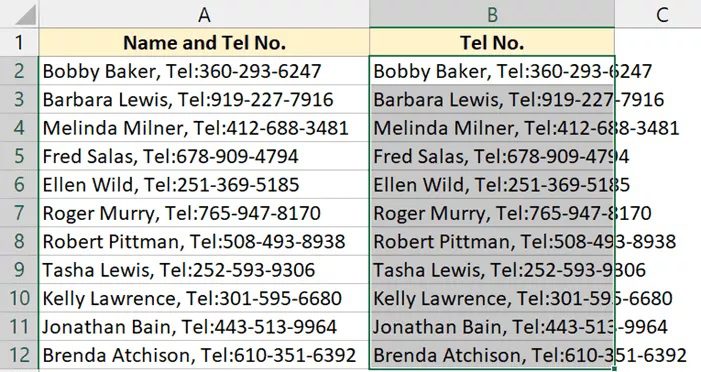
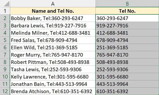
For illustration, I’ve included a data set below that lists the names of my workers along with their phone numbers.
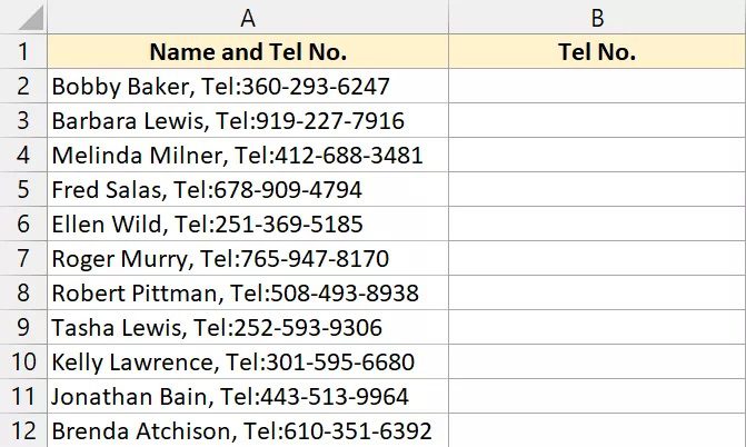
I want to extract the phone number from each cell and nothing else, thus I need to get rid of everything that comes before the phone number.
I need to search for a pattern that I can use to eliminate anything before the phone number, like with most Excel data-cleaning techniques.
It is the text string “Tel:” in this instance.
Therefore, all I have to do is locate the string “Tel:” in each cell and delete anything that comes before it (including it).
Although you could create a complex formula in Excel to accomplish this, let me demonstrate a pretty clever solution by using the Find and Replace method.
The procedures to eliminate all the text before a certain text string are as follows:
- Data from column A should be copied to column B. By doing this, I will still retain the original data in column A while getting the outcome in column B.
- Choose every cell in column B.
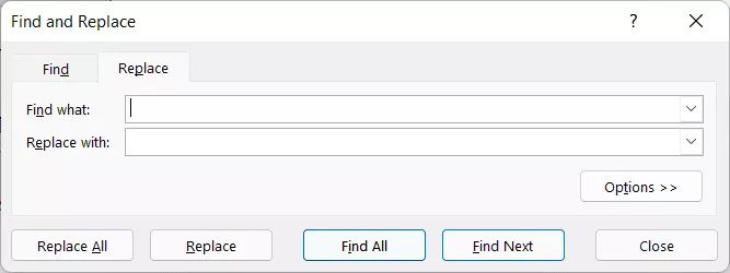
- Press the H key while holding down the Control key (Command + H on a Mac). The Find and Replace dialogue box will then be shown.
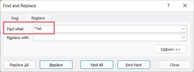
- Enter *Tel: in the “Find what” area.
- Empty the “Replace with” field.
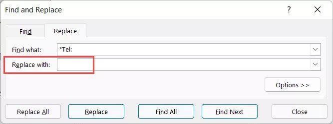
- Select Replace All.
The aforementioned methods would eliminate anything that came before the string “Tel:” leaving you simply with the phone number.
How does that function?
I used the asterisk (*) wildcard character in the aforementioned example.
I inserted an asterisk before the string “Tel:” and used it in the “Find what” section because I wanted to eliminate everything to the left of it.
In Excel, a wild card character known as an asterisk (*) can stand in for any number of characters.
This implies that if I ask Excel to locate “*Tel:” it will search each column for the string “Tel:” regardless of its location, and if it finds the string there, it will take everything up to that point into account when replacing the text.
And because I didn’t replace this with anything (by leaving the “Replace with” box empty), it just deletes the contents of the cell up to that string.
This implies that everything preceding that text string, including that string itself, is eliminated, leaving me with only the characters that follow that text string.
Excel tutorials
5. Eliminate all left-side text (and keep the numbers)
You could occasionally come across a data collection with text and numbers combined in a single cell, as seen below, and want to get rid of all the text while keeping the numbers solely.
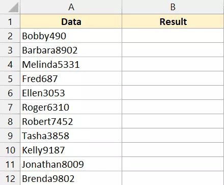
There is an easy formula to use for this.
The formula to eliminate all the text from the space to the left of the numbers, leaving only the string’s numerical component, is shown below.
=RIGHT(A2,LEN(A2)-MIN(IFERROR(FIND({0,1,2,3,4,5,6,7,8,9},A2),LEN(A2)))+1) 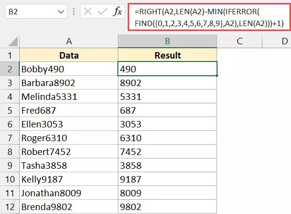
The text in the left-hand portion of the cell would be eliminated by the method above, leaving only the numbers.
Let me now briefly explain how this formula functions.
The formula’s FIND(0,1,2,3,4,5,6,7,8,9, A2) clause would search for these 10 numbers in the cell and would then return an array of their locations.
For instance, the outcome of this formula for sale A2 would be (8,#VALUE!,#VALUE!,#VALUE!,6,#VALUE!,#VALUE!,#VALUE!,7).
As you can see, it produces 10 values, each of which corresponds to a certain number’s location within a cell.
The initial value returned is 8, and as the cell lacks the digit 1, a Value error is issued since the digit 0 occurs in the eighth place.
Similar to this, each digit is examined, and if it is present in the cell, a number is returned; otherwise, the value error is returned.
Now that this FIND formula is included within the IFERROR formula, we receive something more significant in place of the value error.
When it locates the digit in the cell in this instance, the IFERROR formula will return a number. If it does not, it will return the cell’s maximum character length (which is done using the LEN formula)
Excel tutorials
This is done to ensure that the IFERROR formula would still return a digit that could be utilized in the formula if there were cells with no numbers (else it would have returned an error).
I’ve now used the MIN function to get the array’s minimal value using these arrays of integers. This would inform me of the cell’s initial location for the numbers.
For instance, if I typed 6 into cell A2, it would indicate that the text portion of the cell finishes at character number 5, and the numbers start at character number 6.
I need to know how many letters I need to delete from the left now that I know where the numbers in the cell begin.
To do this, I once more used the LEN function to determine the total number of characters in a cell, and then I deducted the outcome of the main function from this to determine the number of text characters in the left cell.
Because I want to omit the cell’s first number, you’ll see that I’ve also removed 1 from the calculation (if I hadn’t, the formula would also remove the text and the cell’s first number).
Lastly, I have used the RIGHT function to remove all of the text characters from the left by extracting all of the numbers from the right.
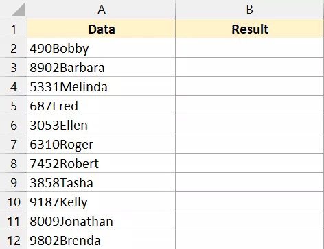
7. Take Off Every Number to the Left
I demonstrated in the previous part how to eliminate all the text characters from the left so that the cell’s sole contents are its numbers.
But what if the circumstances were different?
What if I have a data set like the one below where I want to maintain all the text characters but delete all the numbers from the left?
With a few modifications, we can use a similar formula.
The algorithm to eliminate all the numbers on the left so that you just see the cell’s text is shown below.
=MID(A2,MIN(IFERROR(FIND({"a","b","c","d","e","f","g","h","i","j","k","l","m","n","o","p","q","r","s","t","u","v","w","x","y","z"},LOWER(A2)),LEN(A2))),1000) 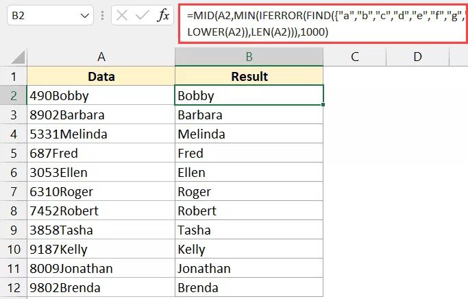
The idea is precisely the same even if this formula could appear larger and a little frightening than the previous one.
The FIND function was employed in this formula to determine the placement of each of the 26 alphabets used in the English language.
The formula’s FIND section locates each of the 26 alphabets by checking the cell and returning the results.
Because the alphabet I’m using in the FIND formula is lowercase, you’ll also see that I used LOWER(A2) rather than A2.
The fine formula was then included in IFERROR so that, in the event that it is unable to locate a certain alphabet, it returns the length of the content in the cell as opposed to the value error (which is given by the LEN formula).
In order to ensure that I would still receive a numeric value if I had a cell with simply numbers and no text, I did this.
The minimal location at which the text begins was then determined using the MIN function.
This would enable me to divide the cell’s content to get rid of all the numbers on the left and preserve the text section while still knowing where the numbers finish and the text begins.
Knowing where the text characters in the cell begin has allowed me to utilise the MID function to extract everything from that point onward.
Please take note that I have set the mid function to extract 1000 characters; however, if your cell has less characters, just that many characters will be extracted.
These are a few instances in which we have eliminated characters from the left in an Excel cell.
I’ve demonstrated formulae for removing a certain amount of characters from the left or characters depending on a delimiter.
I also demonstrated how to eliminate all the characters to the left of a certain string by using a straightforward search and replace method.
Finally, I demonstrated two formulae that you may use to delete either the text or just the numbers from the left.
I hope you learned something from this Excel tutorial.