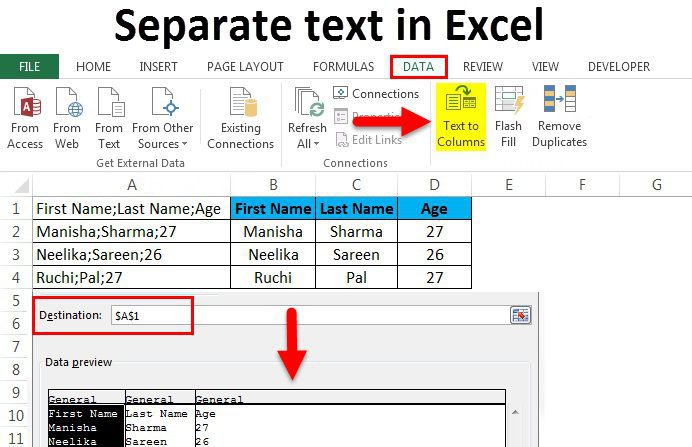
Excel: Separate Text and Numbers (4 Easy Ways):

There are instances when text and numeric data are present in the same cell, and you may need to divide the data into different compartments for the text and the numbers.

There isn’t a built-in way to achieve this directly, but you can utilize various Excel features and formulae.

I’ll demonstrate four Quick and easy ways to separate text and numbers in Excel in this article.

Let’s start now!

This instruction explains:

1. Using Flash Fill, separate text and numbers 2. Use a Formula to Separate Text and Numbers 3. Using VBA, separate text and numbers (Custom Function) 4. Power Query: Separate Text and Numbers

Using Flash Fill, separate text and numbers:

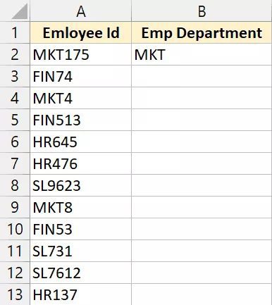
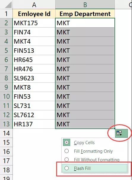
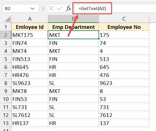
In column A of the personnel data below, the employee’s department is indicated by the first few alphabets, and the following numbers show the employee number.

I want to divide this data into two independent columns, one for the text and one for the numbers (columns B and C).
Using Flash Fill is the first technique I’ll demonstrate for separating text and numbers in Excel.
The Excel 2013 feature called Flash Fill finds patterns based on user input.
Therefore, if I manually enter the desired outcome in column B, Flash Fill will attempt to recognize the pattern and provide me with the development for every cell in that column.
The procedures to remove the text from the cell and place it in column B are as follows:

1. Choose cell B2
2. Manually type MKT into cell B2 to represent the anticipated outcome.

3. Set the cursor to the bottom right corner of the selection when cell B2 is chosen. The cursor morphs into a + sign, as you can see (this is called Fill Handle)

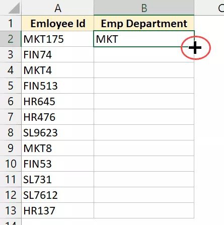
4. Drag the Fill Handle while continuing to press the left mouse/trackpad key to fill the cells. If all of the cells have the same text, don’t worry.

5. Select “Flash Fill” by clicking on the Auto Fill Options button.

6. The text portion would be removed from the cells in column A using the aforementioned processes, and the result would appear in column B.

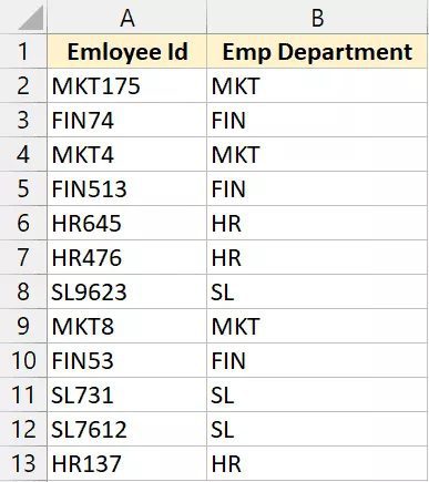
Be aware that Flash Fill could occasionally be unable to recognize the proper pattern. In these situations, it would be advisable to put the anticipated outcome in two or three cells, fill the column with the Fill Handle, and then apply Flash Fill to the data.

The numbers in column C may be extracted using the same procedure. All you have to do is type the anticipated outcome in cell C2 (step 2 in the process laid out above)

Remember that the Flash Fill result is static and won’t change if the original data in column A is changed. Use the formula approach we’ll cover next if you want the outcome to be dynamic.

Use a Formula to Separate Text and Numbers:

I want to use a formula to extract only the text portion and put it in column B and to remove the numerical amount and put it in column C from the employee data in column A below.

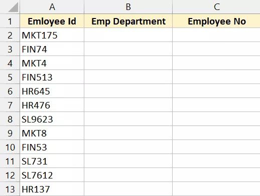
I cannot use the LEFT or RIGHT function to extract only the text piece or the numeric portion since the data is inconsistent (i.e., the alphabets in the department code and the numbers in the employee number are not of constant length).

The formula that will just extract the text from the left is shown below:

=LEFT(A2,MIN(IFERROR(FIND({0,1,2,3,4,5,6,7,8,9},A2),""))-1)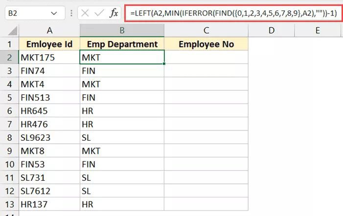

The equation that will pull every integer from the right is shown below:

=MID(A2,MIN(IFERROR(FIND({0,1,2,3,4,5,6,7,8,9},A2),"")),100)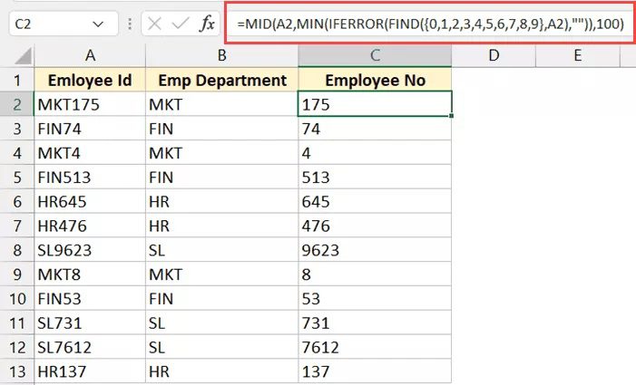

How does this equation function?

First, allow me to describe the algorithm we employ to separate the text portion on the left.

=LEFT(A2,MIN(IFERROR(FIND({0,1,2,3,4,5,6,7,8,9},A2),””))-1)

The formula’s FIND clause determines where the numbers 0 to 9 are located in cell A2. If that digit is located in cell A2, the location of that digit is returned. If what cannot locate that digit, the value error (#VALUE!) is returned.
It produces the following result for cell A2:
{#VALUE!,4,#VALUE!,#VALUE!,#VALUE!,6,#VALUE!,5,#VALUE!,#VALUE!}

1. It returns #VALUE for 0! as cell A2 does not contain this digit.
2. Since the first instance of 1 appears in cell A2 at position 4, it yields 4 for the value 1.
3. and so forth.

The IFERROR function is then used to enclose the FIND formula, eliminating all value mistakes but keeping the numbers intact.

The results are shown as follows:

{“”,4,””,””,””,6,””,5,””,””}

The MIN function then iterates through the result, as mentioned earlier, and provides us with the result’s minimal value. The minimum value indicates where the numerical value starts in the cell since each number in the array indicates where the corresponding number should be in the collection.

Knowing where the numerical values begin allows us to extract everything before this place using the LEFT function (which would be all the text in the cell).

Similarly, with a slight modification, you can extract all the numbers following the text using the same algorithm. Use the MID function to remove everything starting from the first digit when removing numbers when we are aware of that place.

What if the order of the numbers and text is inverted, with the numbers coming first and the text following, and we wish to separate the two?

The same reasoning still applies, with one slight modification: to get the location of the last digit in this cell, you must use the MAX function rather than locating the minimal value, which gives us the position of the first digit in the cell. Once you have it, you may split the numbers and text using the LEFT or MID functions.

Text and Numbers Can Be Separated Using VBA (Custom Function):

While you may use the formulae above to split the text and numbers in a cell and extract these into various compartments, if this is something you need to do frequently, you also have the choice to construct your custom function using VBA.

Making your function would be much simpler (with just one process that takes only one argument).

To make this custom function VBA code available in your Excel workbooks, you may store it in the Personal Macro Workbook.

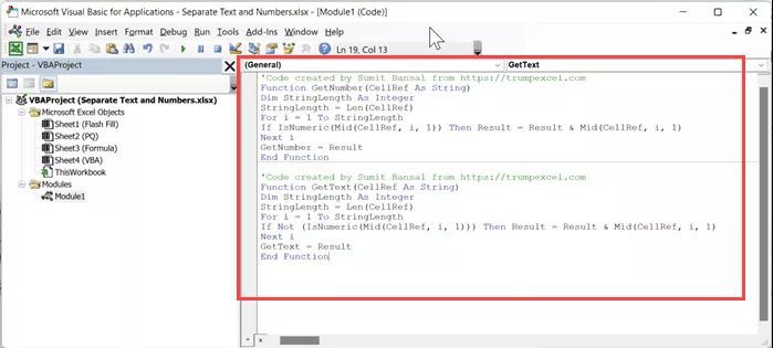
The VBA code that could be used to build the function “GetNumber” below would extract all of the numbers from the cell using the cell reference as the input parameter.

'Code created by Sumit Bansal from https://trumpexcel.com
'This code will create a function that can separate numbers from a cell
Function GetNumber(CellRef As String)
Dim StringLength As Integer
StringLength = Len(CellRef)
For i = 1 To StringLength
If IsNumeric(Mid(CellRef, i, 1)) Then Result = Result & Mid(CellRef, i, 1)
Next i
GetNumber = Result
End Function

'Code created by Sumit Bansal from https://trumpexcel.com
''This code will create a function that can separate text from a cell
Function GetText(CellRef As String)
Dim StringLength As Integer
StringLength = Len(CellRef)
For i = 1 To StringLength
If Not (IsNumeric(Mid(CellRef, i, 1))) Then Result = Result & Mid(CellRef, i, 1)
Next i
GetText = Result
End Function

3. The Project Explorer would be on the left of the Visual Basic editor that would launch. This would provide the names of your current Excel workbook and worksheets. If you cannot see this, select Project Explorer from the menu’s View option.

4. Choose any of the sheet names (or any other object) for the workbook where this function will be added.

5. In the top toolbar, select Insert, and then select Module. By doing so, a new module will be added to that worksheet.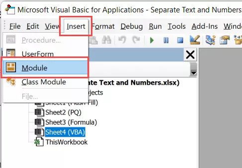

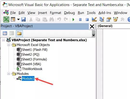
6. The module icon in “Project Explorer” should be double-clicked. The module code window will then be opened.

7. The module code pane will now display the custom function code that was just copied.

8. Shut off the VB Editor.
Using the techniques mentioned earlier, we introduced the custom function code to the Excel spreadsheet.
Now, you may use the worksheet functions =GETNUMBER and =GETTEXT just like any other.

Note: You must save the file as a Macro Enabled file after you have the macro code in the module code box (with the .xlsm extension instead of the .xlsx extension)

It would be more effective if you copied the VBA scripts for building these custom functions and saved them in your Personal Macro Workbook if you frequently needed to separate text numbers from cells in Excel.

This lesson I previously produced will teach you how to construct and utilize a personal macro workbook.

You may utilize these functions on any Excel workbook on your machine once you have them in the Personal Macro Workbook.

One thing to keep in mind is that you must add the prefix =PERSONAL.XLSB! to the function name when employing functions that are saved in Personal Macro Workbook. For instance, if I have the code for the function GET NUMBER stored in the postal macro workbook and I want to utilize it in an Excel workbook, I must use =PERSONAL.XLSB! GET NUMBER(A2)

Power Query: Separate Text and Numbers:

I’m slowly starting to love Excel’s Power Query tool.

If Power Query is already a part of your workflow and you have a data set where you wish to divide the text and numbers into distinct columns, Power Query can accomplish it in a few clicks.

If you wish to utilize Power Query to change Excel data, you need to turn the Excel data into an Excel Table (or a named range).

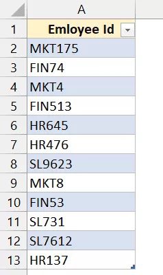
I’ve included an Excel table with the data below that I want to divide into distinct columns for the text and numbers.

The steps to achieve this are as follows:

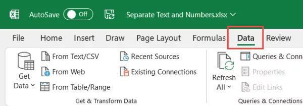
1. In the Excel Table, choose any cell.
2. Choose the Data tab from the ribbon.

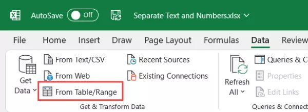
3. Click the “From Table/Range” link under the Get and Transform group.

4. Select the column from which you wish to split the numbers and text in the Power Query editor that appears.

5. Open the Power Query ribbon and choose the Transform tab.

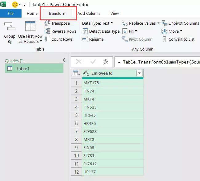
6. Select “Split Column” from the menu.

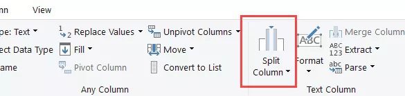
7. Select “By Non-Digit to Digit” from the option.

8. As you can see, the column has been divided into two, one of which contains only the text, and the other of which only contains the numbers.

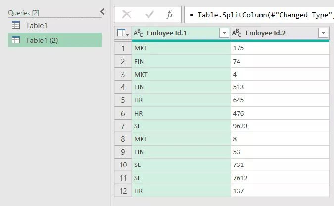
9. [Optional] If desired, you may alter the column names.

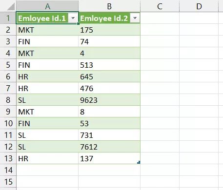
10. After selecting the Home tab, click Close and Load. This will create a new sheet and produce an Excel Table for us.

The procedures mentioned above would extract the data from the Excel Table we had initially, split the column using Power Query to divide the text and numeric components into two different columns, and then return the output in a new sheet within the same workbook.

In step 7, we selected the “By Non-Digit to Digit” option, which causes splits each time a character changes from a non-digit to a digit. Use the “By Digit to Non-Digit” option if your dataset contains numbers first, then text.

Let me now highlight the finest feature of this approach. The output Excel Table is linked to your original Excel Table, which serves as the data source.
As a result, you need not start over if your original data changes. You may right-click on any cell in the output Excel Table and select Refresh.

When running in the background, a power query would verify the complete original data source, do all of the changes we made in the previous phases, and update the data in your output results.

Power Query shines in this situation. You may use Power Query to perform a transformation once and build up a process if you frequently need to convert a batch of data. The original data source and the output data would be connected by Excel, which would also keep track of all the procedures you used to change the data.

The result will be available in a few seconds if you replace your old data with the new data set and refresh the query. In Power Query, you can also easily switch the source from the current Excel table to another Excel Table (in the same or different workbook).
These are the four straightforward methods you may use in Excel to separate numbers and text. Flash Fill or the formula technique is preferable if this is a once-in-a-while activity.
And if you find yourself needing to do this very frequently, I advise you to consider either the Power Query way or the VBA method, where we establish a custom function.

I hope you learned something from this Excel tutorial.

See Our More Excel Tutorial