How Can Drop-Down Lists Be Removed From Excel? Simple Steps!

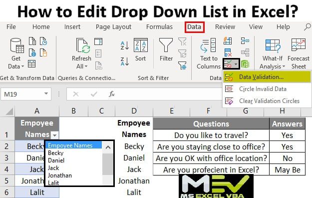
Since I first discovered them, Excel drop-down lists have been a favorite of mine. It expedites data entry. Additionally, it enables me to produce interactive dashboards and reports (where a user can choose an option from the drop-down in the entire dashboard updates).

It’s also a helpful tool for when I share my files with others because I can prevent data from entering some cells and just permit drop-down selections.

But occasionally you might need to get rid of the drop-down from your Excel file.

This can be the case if you no longer require the drop-down or wish to enter something different from the choices offered.

I’ll rapidly demonstrate how to remove a drop-down in Excel in this lesson. I’ll also explain how to delete every drop-down menu from your excel file instantly.

This instruction explains:

Why Are Drop-down Lists Removed From Excel?

Excel: Remove Particular Drop-down Lists

2.1. Data Validation Dialog Box Use

2.2  Making use of the Clear All button

2.3 Copy-Paste Technique

Eliminate every drop-down list from the worksheet.

3.1 according to the same list

3.2 Using the various Lists

Maintain the Drop-Down List While Allowing All Entries (No Error Message)

Why Are Drop-down Lists Removed From Excel?

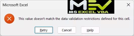
The main reason individuals desire to remove a drop-down list in Excel is so they can input different text from what is already there.

A message will appear if you attempt to enter something different into a cell that has a drop-down list in it (as shown below).

Another frequent excuse is when you want to redesign the drop-down list but first remove all of the ones that are currently in the worksheet.

Excel: Remove Particular Drop-down Lists:

I’ll start by demonstrating how to delete a particular drop-down list from the spreadsheet.

It would be best to choose the drop-downs (all the cells with multiple drop-downs) you want to delete for this method to function.

In the section after this one, I’ll also demonstrate how to eliminate every drop-down in the spreadsheet.

Data Validation Dialog Box Use:

I have developed drop-down lists in the adjacent cell (column B) that would display the department names. Below, I have the Employee name data set in column A.

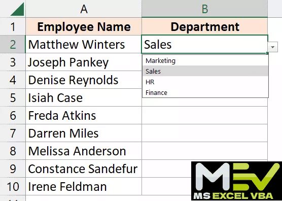
I want to remove every drop-down in column B from this data.

The methods for using the data validation dialogue box to remove the drop-down from column B are listed below.

Choose the cells with the drop-down menu that you want to remove.
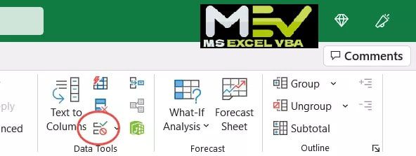
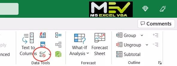
Choose the “Data” tab.

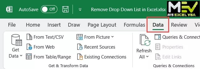
3. Select “Data Validation” by clicking the icon in the “Data Tools” group. This will bring up a dialogue window for data validation.

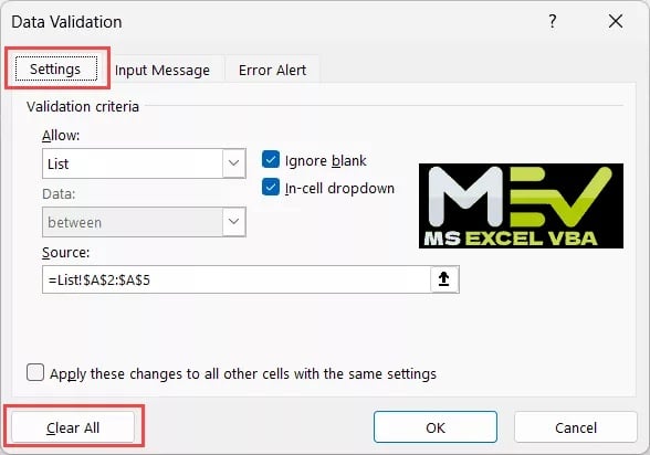
4. Make sure the Data Validation dialogue box’s “Settings” tab is chosen.
5. Press the “Clear All” button.

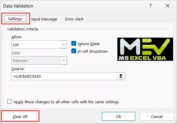
6. Hit “OK”

Since a drop-down list is a kind of data validation rule, the aforementioned actions would also clear any data validation rules that were present in the selected fields.

Keep in mind that: the value would still be there in the cell if you had previously made selections using the drop-down lists. 
The drop-down list would be the only thing gone.

Pro Tip:
The keyboard shortcut ALT + A + V + V can be used to open the data validation dialogue box (press these keys one after the other)

Making use of the Clear All button:

I’ll start by demonstrating how to delete a particular drop-down list from the spreadsheet.

It would be best to choose the drop-downs (all the cells with multiple drop-downs) you want to delete for this method to function.

In the section after this one, I’ll also demonstrate how to eliminate every drop-down in the spreadsheet.

Instead, you can choose the ribbon’s “Clear All” option.

I’ve included a data set below with the names of the employees in column A and a drop-down menu in column B. (where the drop-down list shows the department names of the employees).

The ‘Clear All’ approach can be used to remove the drop-down menus from the cells as seen below:

The cells with the drop-down that you want to remove should be selected.
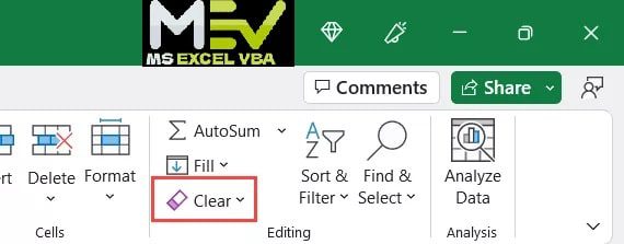
Choose the “Home” tab.
Select “Clear” from the Editing group’s menu by clicking it.

4. Select “Clear All” from the menu options that appear.

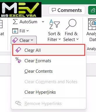
The aforementioned procedures would empty the cells of everything (including the drop-down list, any values in the cells, as well as any formatting applied to the cells).

This approach is more suited when you wish to start again and eliminate everything from the cells to do so.

Pro Tip:
You can also press ALT + H + E + A to completely clear the contents of the chosen cells
(press these keys one after the other)

Copy-Paste Technique:

Drop-down list formatting in Excel is identical to cell formatting. This enables you to copy and paste a drop-down list with only a few simple clicks.

In the opposite case, what would eliminate the drop-down list if you copied and pasted a cell with no drop-down list over a cell with one (as the formatting and the data validation rules of the copied cells are applied the destination cell ref)

Below is a data set from which I want to delete the drop-down lists in column B.

Here are the steps to remove the drop-down menu using a straightforward copy-and-paste technique:

Choose a worksheet cell that is empty and doesn’t have a drop-down menu.
Copy this cell by using the keyboard shortcut Control + C in Windows or Command + C on Mac (or by right-clicking the cell and selecting Copy).
Choose the cells containing the drop-down list you want to delete.
Select the desired cells, then pick the Paste option from the shortcut menu that appears when you right-click (Control + V or Command + V).

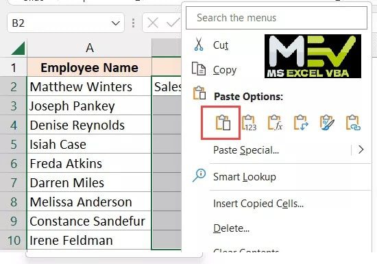
The drop-down list would be removed from the chosen cells using the aforementioned processes.

This approach has the downside of copying the formatting from the cell that we copied in step 2 and remove all formatting from the cells.

Eliminate every drop-down list from the worksheet.

I demonstrated three ways to get rid of the drop-down list from the chosen cells in the section above.

You must be aware of the locations of these drop-down lists to select those cells before removing them for those techniques to function.

In this section, I’ll demonstrate how to delete every drop-down list on the worksheet without picking it out individually from each cell.

There are two situations in which you can apply this technique:

When you wish to eliminate every drop-down list made using the same source list in the worksheet, then.
When you want to delete each drop-down list, regardless of where they came from.

According to the same list:

In the data set below, I’ve generated drop-down lists in two columns (columns B and E) using the same source list (so all the cells show the same data in the drop-down menu)

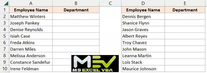
Moreover, I want to get rid of both of these drop-down menus.

To remove all the drop-down lists at once, follow these steps:

Choose any cell that contains the drop-down you want to remove.
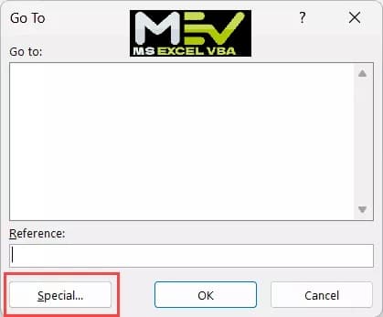
You can alternatively go to the “Home” tab, click on the “Find & Select” option in the Editing group, and then click on the “Go To” option. Pressing the F5 key on your keyboard will bring up the Go To dialogue box.
Click the “Special” button in the “Go To” dialogue box.

4. Select the ‘Data Validation’ radio button in the ‘Go To Special’ dialogue box.

5. Within the Data Validation option, choose the ‘Same’ option.

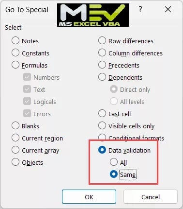
6. Input OK.

All cells with drop-down lists that use the same source list as the cell we picked in step 1 will be selected by the aforementioned steps.

Here are the procedures to remove the drop-down list once we have picked every cell that contains one.

7. Choose the “Data” tab.

8. Select a “Data Validation” icon from the “Data Tools” group.

9. Make sure the Data Validation dialogue box’s Settings tab is chosen.
10. Press the “Clear All” button.

11. Click “OK”

The above steps would a remove of all the drop-down menu that is based on the same list as the one in the cell that was selected in Step 1.

Using the various Lists:

You can use the procedures in this section if you want to delete all the drop-down lists in the worksheet at once, regardless of their source list.

You can alternatively go to the “Home” tab, click on the “Find & Select” option in the Editing group and then click on the “Go To” option. Pressing the F5 key on your keyboard will bring up the Go To dialogue box.
Select “Special” from the menu. What will then display the Go To Special dialogue box?
Choose the “Data Validation” menu item.
Ensure that the ‘All’ option is chosen.

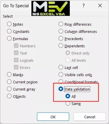
5. Select OK. This will pick out all the cells where data validation rules are in effect.
6. Go to the Data tab.

7. Select the “Data Validation” icon from the “Data Tools” group.

8. Ensure the Data Validation dialogue box’s “Settings” tab is chosen.

9. Press the “Clear All” button.

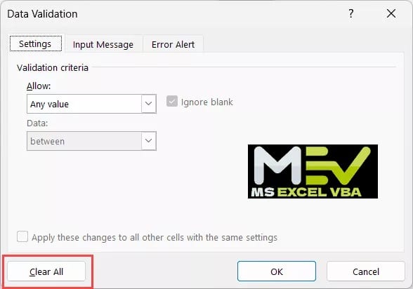
10. Enter OK.
All the drop-down lists in your worksheet would be deleted using the methods mentioned.

The benefit of this approach is that you do not need to be aware of the fact that all cells include drop-down menus. This is handled for you by the ‘Go To Special’ option.

Caution: It's crucial to keep in mind that the methods mentioned earlier would eliminate all forms of data validation criteria from the worksheet. 
The most popular data validation option is a drop-down list, although many users also utilize data validation rules that don't require establishing a drop-down menu (such as restricting data entry between two numbers or two dates). Any cell that has any data validation rule applied to it would be selected by the processes mentioned above 
(not just the drop-down lists)

Maintain the Drop-Down List While Allowing All Entries (No Error Message)

Users will occasionally accept the retention of drop-down menus if the cells permit data entry by hand.

For instance, if I wish to add “NA” or “Not Assigned” for one person in a drop-down list that displays department names for employees, I won’t be able to because it isn’t a part of the list.

But what if there was a method to maintain the drop-down list while also allowing you to enter values that aren’t on it?

I’ll demonstrate how to accomplish it for you.

In the data set below, column B contains drop-down lists that I want to maintain while also allowing me to manually add data into these cells.

The steps are as follows:

Choose the cells that have drop-down menus.
Go to the Data tab.
Select the “Data Validation” icon from the “Data Tools” group.

5. Select of the “Error Alert” tab in the Data Validation dialogue box.

6. The checkbox for “Show error alert if invalid data is entered” should be unchecked.

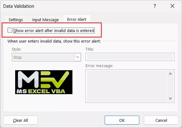
7. Enter Ok

Once you’ve completed the aforementioned procedures, you won’t see the error message prompt while entering any data in the cell.

Additionally, you can enter data by selecting items from the drop-down list concurrently (so the best of both worlds).

I’ve shown you several techniques in this tutorial for deleting drop-down menus from Excel cells. Using the built-in clear all option in the data validation dialogue box or the “Clear All” option will erase everything, including the drop-down lists if you wish to remove it from certain cells.

I’ve also discussed how to eliminate every drop-down list from a worksheet (based on the same list or irrespective of the source lists)

I hope you learned something from this Excel tutorial.

See Our More Excel Tutorial