How to Apply a Formula to the Entire Column in Excel (5 Easy Ways)

The heart and soul of an Excel spreadsheet are its formulas. Additionally, you typically don’t require the formula in just one or a few cells.

The formula would often need to be applied to a full column (or a large range of cells in a column).

Excel also provides you with several options for doing this with only a few clicks (or a keyboard shortcut).

Let’s examine these approaches.

This instruction explains:

1. By pressing the AutoFill to handle twice 2. Drag the AutoFill Handle to fill 3. Fill Down Option (located in the ribbon) use 3.1 Fill Down being added to the Quick Access Toolbar 4. Keyboard shortcuts 5. Array Formula Utilization 6. By Pasting the Cell as a Copy

1. By pressing the AutoFill to handle twice

The usage of this straightforward mouse double-click technique is one of the simplest ways to apply a formula across a whole column.

Consider the following dataset, where you want to determine the commission for each sales representative in Column C (where the commission would be 15% of the sale value in column B).

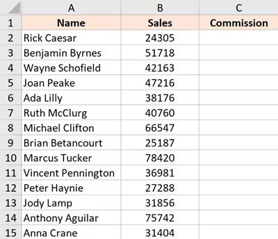
For this, the equation would be:

=B2*15%

The steps for applying this formula to all of column C are listed below:

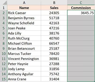
Put the following equation in cell A2: =B2*15%
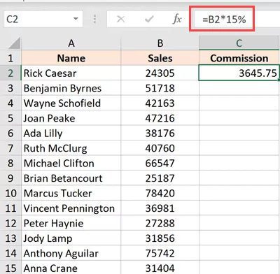
When a cell is selected, a tiny green square will appear in the bottom-right corner of the selection.
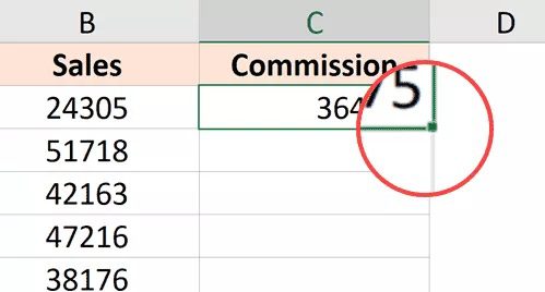
The little green square with the pointer over it. The cursor transforms to a plus sign, as you will see (this is called the autofill handle)
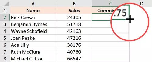
Press the left mouse button twice.

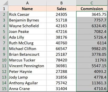
The aforementioned actions would automatically fill the column up to the cell containing the data from the neighboring column. The formula would be applied to cell C15 in our case.

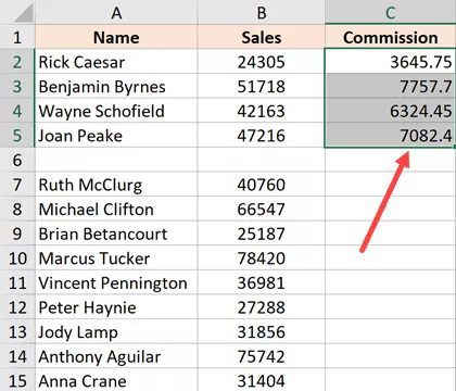
The neighboring column must be empty of any data and include no blank cells for this to function. For instance, if cell B6 in column B is blank, the auto-fill double click would only apply the formula up to cell C5.

It’s the same as manually pasting the formula when you use the autofill handle to apply it to the full column. This implies that the formula’s cell reference would adjust appropriately.

If the reference is absolute, for instance, it would not change when the formula is applied to the column; but, if the reference is relative, it would change as the formula is applied to the cells below.

2. Drag the AutoFill Handle to fill

The aforementioned double-click technique has the drawback of stopping as soon as it reached a blank cell in one of the neighboring columns.

You may also manually drag the fill handle to apply the formula to the column if you just have a little amount of data.

The procedures are as follows:

Put the following equation in cell A2: =B2*15%
When the cell is selected, a tiny green square will appear in the bottom-right corner of the selection.
The little green square with the pointer over it. The cursor transforms to a plus sign, as you will see.
Holding down the left mouse button, move it to the cell where you wish to apply the formula.
After finishing, release the mouse button.

3. Fill Down Option (located in the ribbon) use

Using the fill-down feature in the ribbon is an additional method for applying a formula to a whole column.

You must first choose the cells in the column where you want the formula to appear for this approach to function.

The fill-down approach is used as follows:

Put the following equation in cell A2: =B2*15%
To apply the formula, select every cell (including cell C2)
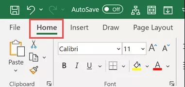
On the Home tab, click
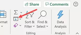
Click the Fill icon in the editing group.
Select “Fill down”

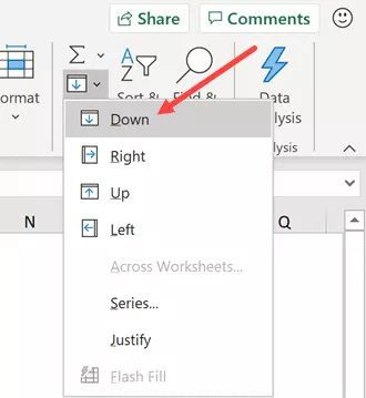
The previous stages would use cell C2’s formula to fill in all the chosen cells.

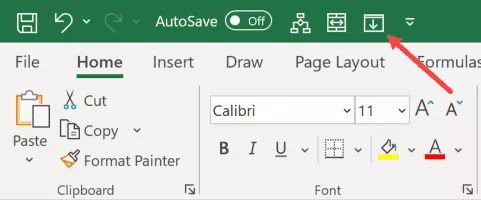
3.1 Fill Down being added to the Quick Access Toolbar

If you frequently need to utilize the fill-down option, you may put it on the Quick Access Toolbar so that you can access it with just one click and that it is always visible on the screen.

Go to the “Fill Down” option, right-click on it, and then select “Add to the Quick Access Toolbar” to add it to the Quick Access Toolbar (QAT).

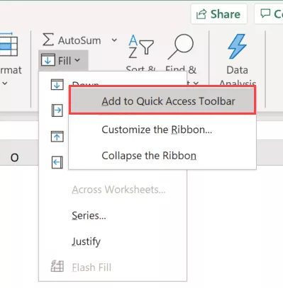
The ‘Fill Down’ symbol will now show up in the QAT.

4. Keyboard shortcuts

You may also use the keyboard shortcut shown below to get the fill-down feature if you prefer that method:

CONTROL + D (hold the control key and then press the D key)

The steps to filling down the formula using the keyboard shortcut are as follows:

Put the following equation in cell A2: =B2*15%
To apply the formula, sever every cell (including cell C2)
Press the D key while holding down the Control key.

5. Array Formula Utilization

To apply a formula to the full column, you may alternatively use the array formula technique if you’re using Microsoft 365 and have access to dynamic arrays.

Let’s say you wish to determine the Commission in column C using the data set depicted below.

The formula you may use is as follows:

=B2:B15*15%

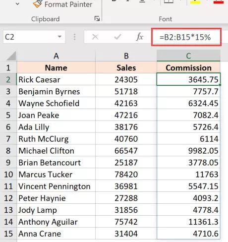
With this array formula, the cell would receive 14 values (one each for B2:B15). However, because we are using dynamic arrays, the outcome would not be limited to a single cell but would instead overflow and cover the full column.

Remember that not every situation allows for the application of this formula. Because our formula utilizes the input value from a neighboring column and has the same number of cells (14 in this example) as the column in which we want the output, it functions correctly in this situation.

However, if that’s not the case, then perhaps this isn’t the ideal method for copying a formula to the full column.

6. By Pasting the Cell as a Copy

Another easy and common way to apply a formula to the whole column (or certain cells within the whole column) is to simply copy the formula-containing cell and paste it over the cells you need it in the column.

The procedures are as follows:

Put the following equation in cell A2: =B2*15%
Use the keyboard shortcut Control + C in Windows or Command + C on Mac to copy the cell.
Select each cell where the same formula should be applied (excluding cell C2)
Copy the cell, then paste it (Windows: Control + V, Mac: Command + V).

This copy-paste technique differs from all the conversion techniques above it in that you may select to just paste the formula using it (and not paste any of the formatting).

For instance, if cell C2 had a blue cell color, all the techniques shown thus far (except the array formula approach) would paste the formatting (such as the cell color, font size, and bold/italics) together with the formula to the entire column.

Use the following steps if you simply want to apply the formula and not the formatting:

Put the following equation in cell A2: =B2*15%
Use the keyboard shortcut Control + C in Windows or Command + C on Mac to copy the cell.
Select each cell where the same formula should be applied.
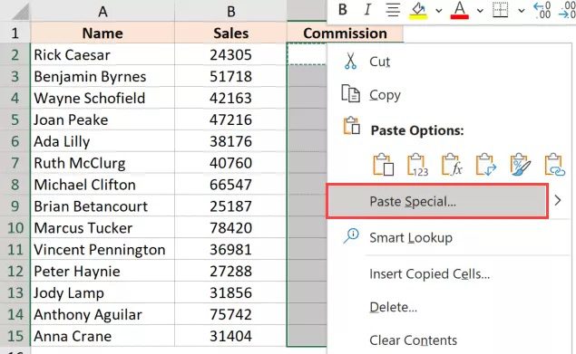
Select using the right mouse button.
Toggle to “Paste Special” from the list of alternatives that appears.
Select the Formulas option in the “Paste Special” dialogue box.
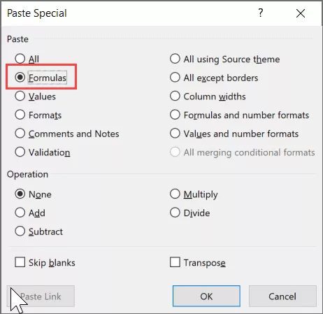
Input OK.