How to Make Text Rotate in Excel Cells (Easy Steps)

One of my responsibilities as a full-time analyst was to  weekly reports for clients and stakeholders.

I had to make sure my reports were simple to read and took up the least amount of screen space (apparently, clients hate scrolling back and forth).

And in such reports, the ability to rotate text was helpful.

When you have a large heading and a little number, it is extremely helpful (as shown below). Due to their slant, the headers in Row 1 take up less space in this example (as compared to when they are horizontal)

I’ll walk you through the process of swiftly rotating text in Excel in this lesson.

This instruction explains: 1. Using the Ribbon Alignment Options, rotate the text 2. Using the Ribbon Format Cells Dialog Box, rotate the text 3. Keyboard Shortcut for Excel Text Rotation 4. Transform the text so that it is once again horizontal (Default State)

1. Using the Ribbon Alignment Options, rotate the text

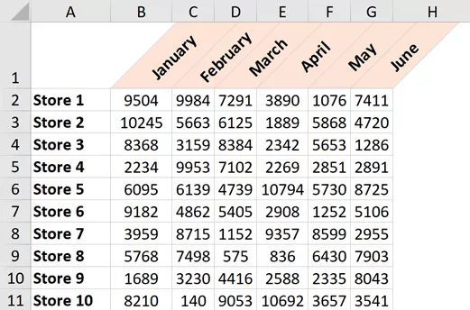
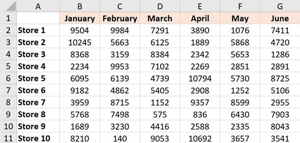
Let’s say you wish to rotate the first row of headers in a dataset like the one below

The steps to rotate the text in the cells are as follows:

1. Choose every cell (that has the headers)
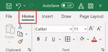
2. On the Home tab, click
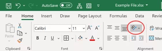
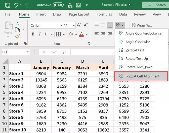
3. Click the “Orientation” icon in the Alignment group.
4. Click the “Angle Counterclockwise” option under the list of available options.

 

By following the steps above, the text in the chosen cells would rotate by 45 degrees.

Additionally, you have the choice to select Rotate Text Up or Angle Clockwise. Although there are additional choices, I don’t utilize them (and not sure if anyone does).

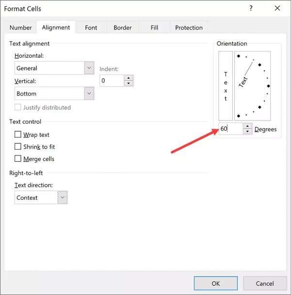
Although there are few possibilities, this is an easy approach to rotating text in a cell. What if, for instance, you want the angle of rotation to be somewhat higher than 45 degrees? (say 60 degrees).

You may accomplish that too, but you’ll need to utilize the approach that follows, which is detailed in this lesson.

2. Using the Ribbon Format Cells Dialog Box, rotate the text

You need to click a few more times, but it takes a little longer and provides you far more control.

Let’s say you wish to rotate the first row of headers in a dataset like the one below.

The procedures are as follows:

1. Choose every cell (that has the headers)
2. On the Home tab, click
3. Click the “Orientation” icon in the Alignment group.
4. Select “Format Cells Alignment” from the menu that appears.
5. Enter the angle by which you wish the text to be rotated in the orientation area.
6. dialogue box closed

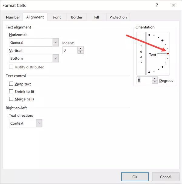
The appropriate alignment can also be obtained by using the mouse to click on the red dot in the Orientation option.

3. Keyboard Shortcut for Excel Text Rotation

Getting accustomed to the shortcut for rotating the text might save you time if you need to do it frequently.

The keyboard shortcut to rotate the text in the chosen cells is listed below.

ALT + H + F + Q + O (press one after the other)

Even though it’s a lengthy keyboard shortcut, it’s still the quickest method if you frequently need to utilize this option.

4. Transform the text so that it is once again horizontal (Default State)

You must return and turn off the current setting if you want to get rid of the rotated text and get the standard horizontal text back (which you can do by clicking on the same option in the ribbon again).

For instance, go to the same option and click on the text again if you have it set to Angle Counterclockwise (it works as a toggle).

Alternatively, you may utilize the Alignment dialogue box (the second technique described in this video), where the orientation degrees should be set to 0.

These are a few techniques for swiftly rotating text in Excel.

I sincerely hope this instruction was helpful.