How to Remove Text in Excel Before or After a Particular Character

You might need to delete the text before or after a certain character or text string while dealing with text data in Excel.

For instance, if you have a person’s name and designation in your data, you might simply want to preserve the name and delete the designation after the comma (or vice-versa where you keep the designation and remove the name).

Sometimes a straightforward formula or a fast Find and Replace can suffice, and other times more complicated formulae or workarounds are required.

In this article,

I’ll demonstrate how to use Excel to delete the text that appears before or after a certain character (using different examples).

So let’s begin with a few straightforward examples.

This instruction explains: 1. Find and Replace to Remove Text Following a Character 2. Using formulas, remove text 3. Use Flash Fill to delete text. 4. Text Removal using VBA (Custom Function)

1. Find and Replace to Remove Text Following a Character

Using Find and Replace and wildcard characters, you may swiftly delete all the words that come after (or before) a certain text string.

Assume you have the dataset depicted below and wish to maintain the text that comes before the comma while removing the designation that follows.

The procedures are as follows:

Data should be copied and pasted from column A to column B. (this is to keep the original data as well)

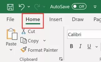
Select the cells in Column B, then select the Home tab.

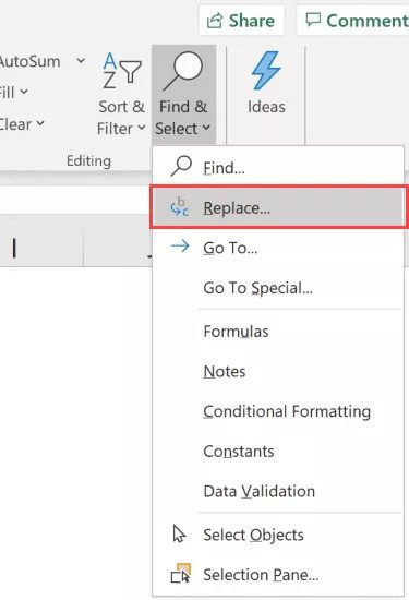
Click the Find & Select button in the Editing group.

Click on the Replace option from the drop-down menu of available choices. The Find and Replace dialogue box will then be shown.

Enter * in the “Find what” area (i.e., comma followed by an asterisk sign)

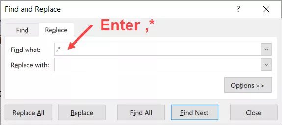
Empty the “Replace with” field.

Select “Replace All” from the menu.

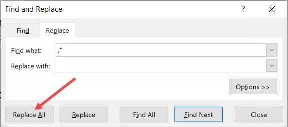
The aforementioned procedures would locate the comma in the data collection and eliminate any text following the comma (including the comma).

It’s a good idea to transfer the text into another column before doing this search and replace operation since doing so replaces the text from the chosen cells. You can also make a backup copy of your data to ensure that the original data is not lost.

How does that function?

The wildcard character * (the asterisk symbol) can stand in for any number of characters.

It recognizes the initial comma in the cell as a match when I use it after the comma (in the “Find what” box) and click the Replace All button.

This is so because the full-text string that follows the comma is regarded as a match for the asterisk (*) symbol.

Therefore, when you click the “replace all” button, the comma and all the content that follows are replaced.

Note:

When there is only one comma in each cell, this strategy works nicely (as in our example). If there are numerous commas, this technique will always locate the first one and then eliminate anything that follows it. To order to change all the content following the second comma while maintaining the first one as is, you cannot use this procedure.

Change the find what field input so that the asterisk symbol appears before the comma (*, rather than,*) if you wish to eliminate all the characters before the comma.

2. Using formulas, remove text

Use Excel’s built-in text formulae if you want greater flexibility over how to identify and replace text before or after a certain character.

Let’s say you want to get rid of all the content that comes after the comma in the data set below.

The formula to achieve this is as follows:

=LEFT(A2,FIND(",",A2)-1)

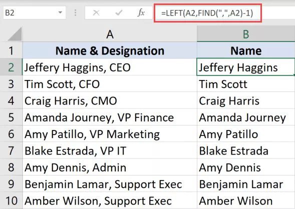
The FIND function is used in the formula above to determine where the comma should be placed in the cell.

The LEFT function then employs this position number to extract all the characters before to the comma. I have deducted 1 from the value returned by the Find formula since I do not want the comma to be a part of the result.

It was an easy situation.

Take one that is a little bit complicated.

Suppose I have this below data set where I want to remove all the text after the second comma.

The equation to do this is as follows:

=LEFT(A2,FIND("!",SUBSTITUTE(A2,",","!",2))-1)

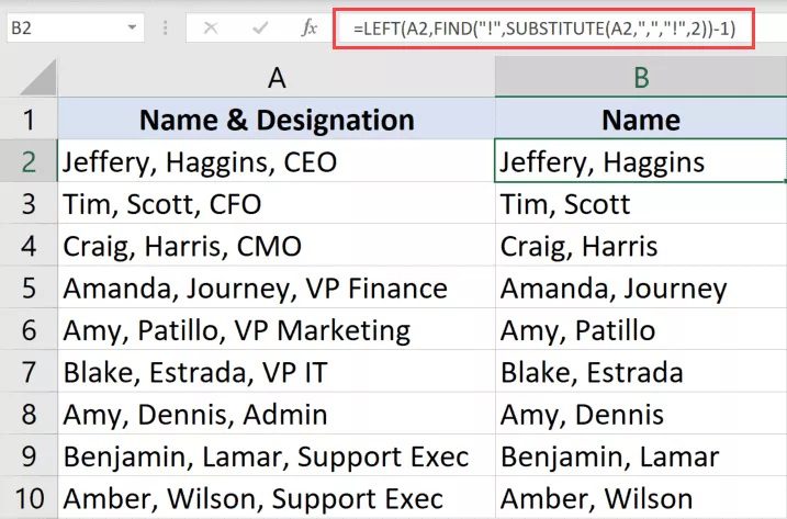
I am unable to extract everything to the left of the first comma in this data set’s numerous commas using the FIND function. I need to locate the second comma somehow, and then I need to remove anything that is to the left of the second comma. I am unable to extract anything to the left of the first comma in this data set using the FIND function since there are several commas in the data. I must determine the second comma’s location in some way before extracting everything to its left.

But what if the data collection has a variable number of commas?

For instance, I need to extract all the content before the final comma from the data set below where some cells have two and others have three commas.

In this instance, I need to locate the last time the comma appears and then remove everything to the left of it.

The equation to accomplish it is given below.

=LEFT(A2,FIND("!",SUBSTITUTE(A2,",","!",LEN(A2)-LEN(SUBSTITUTE(A2,",",""))))-1)

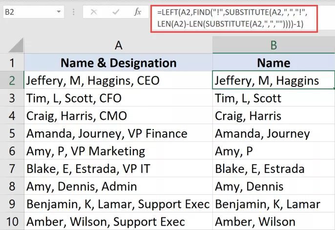
The LEN function is used in the formula above to get both the total length of the text in the cell and the length of the text without the comma.

These two numbers may be subtracted to get the total number of commas in the cell.

I would receive 3 for cell A2 and 2 for cell A4, respectively.

The last comma is subsequently changed to an exclamation point using this value in the SUBSTITUTE formula. Then, using the left function, you may remove everything that is to the left of the exclamation point (which is where the last comma used to be)

3. Use Flash Fill to delete text.

A feature called Flash Fill was added to Excel 2013 and is included in all subsequent iterations.

When you manually enter the data, it finds patterns that are then extrapolated to give you the data for the whole column.

Because of this, if you want to delete the text that comes before or after a certain character, all you have to do is manually type in the desired outcome a few times to demonstrate it to Flash Fairy. Flash Fill will then recognize the pattern and output the desired results.

I’ll provide an illustration to demonstrate this.

The data set where I want to eliminate all the content following the comma is shown below.

To accomplish this with Flash Fill, follow these steps:

In the adjacent column of our data, cell B2, type “Jeffery Haggins” by hand (which is the expected result)
Put “Tim Scott” in cell B3 (which is the expected result for the second cell)
Choose the B2 through B10 range.
On the Home tab, click
Go to the Editing group and select the Fill drop-down menu.
Select Flash Fill.

The results of the aforementioned steps are displayed below:

After choosing the cells in the result column with the keyboard shortcut Control + E, you may also utilize Flash Fill (Column B in our example)

Flash Fill is a fantastic tool that can typically identify the pattern and provide you with the desired outcome. however, occasionally, it could be unable to identify the pattern accurately and provide you with inaccurate results.

Therefore, be sure to verify your Flash Fill findings twice.

You may follow the same procedures to delete the text before a certain character, exactly as we did when removing all the text using flash fill after a particular character. Simply demonstrate to flash fill in the adjacent column how the outcome should seem by using my Internet, and it will take care of the rest.

4. Text Removal using VBA (Custom Function)

Finding the location of a particular character is essential to the idea of eliminating the text before or after it.

Finding the final instance of that character that is excellent requires applying a variety of formulae, as can be seen above.

If you need to perform this task frequently, you may make it easier by using VBA to create a custom function (called User Defined Functions).

Once constructed, this function can be used again. Additionally, it is much simpler and easier to use (as most of the heavy lifting is done by the VBA code in the back end).

The Excel custom function may be created using the VBA code below:

Function LastPosition(rCell As Range, rChar As String)
'This function gives the last position of the specified character
'This code has been developed by Sumit Bansal (https://trumpexcel.com)
Dim rLen As Integer
rLen = Len(rCell)

For i = rLen To 1 Step -1

If Mid(rCell, i - 1, 1) = rChar Then
LastPosition = i - 1
Exit Function
End If
Next i
End Function

Either in the Personal Macro Workbook or a standard module in the VB Editor, you must insert the VBA code. You may use it like you would any other standard worksheet function once you have it present in the workbook.

This function has two inputs:

The cell reference where you’re trying to track down the last instance of a certain character or text string
Your goal is to determine the location of a character or text string.

Consider that you currently have the data set below and would like to just save the text that comes before the last comma.

The equation to accomplish it is given below:

=LEFT(A2,LastPosition(A2,",")-1)

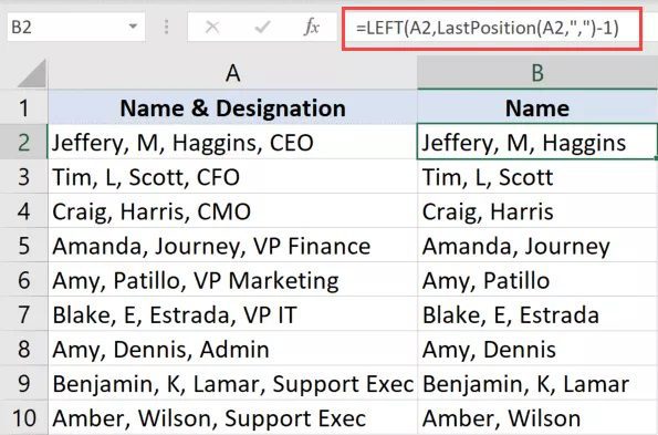
I specifically said to locate the final comma’s location in the formula above. Use it as the function’s second parameter if you wish to determine the location of another character or text string.

As you can see, this is more simpler and shorter than the lengthy text formula we used in the previous part.

You would only be allowed to utilize this custom function in that specific workbook if the VBA code was contained in a module in the workbook. You must copy and paste this code into the Personal Macro Workbook if you wish to utilize it in all of the workbooks on your system.

These are a few of the emails you can use in Excel to rapidly eliminate text that comes before or after a particular character.

Find and replace can be used to complete simple one-time tasks. What if it’s a bit more complicated? In that case, you’ll need to combine many built-in Excel formulae or even make your unique formula using VBA.