Skip to content
LOOKUP
When you need to search a single row or column and find a value from the same point in a different row or column, use the lookup and reference function LOOKUP. Consider the scenario where you are aware of the part number for an automobile component but not the cost.
Summary
In a one-column or one-row range, the Excel LOOKUP function conducts a rough match lookup and returns the corresponding value from another one-column or one-row range. The default nature of LOOKUP makes it beneficial for resolving particular Excel issues.
Purpose
Get back value
Syntax
Arguments
lookup_value -search for the value with lookup value.
lookup_vector -search within a single row or single column.
result_vector -The single-row or single-column set of results.
Version
Excel 2003
Usage notes
Apply the LOOKUP function to obtain a value from the same position in a different one-column or one-row range after looking up a value in a one-column or one-row range. There are two formats for the lookup function: vector and array. The last example below demonstrates the array form, while the remainder of this article discusses the vector form.
The lookup value, lookup vector, and result vector are the inputs the LOOKUP function accepts. The first argument specifies the value to search for, the lookup value. The one-row or one-column range to search is specified by the second argument, the lookup vector. The lookup vector is assumed to be sorted in ascending order by LOOKUP. The third argument, the result vector, represents a one-row or one-column range of results. The resulting vector is not required. LOOKUP searches for a match in the lookup vector when the result vector is supplied and then returns the relevant value from the result vector. LOOKUP returns the value of the match found in the lookup vector if the result vector is not specified.
Because of its built-in default characteristics, LOOKUP can be helpful in some situations. For instance, LOOKUP can locate the final value in a row or column and retrieve an approximate-matched value rather than a position. When performing an approximate match, LOOKUP assumes that the values in the lookup vector are sorted in ascending order. The next smallest value will be matched if LOOKUP is unable to locate a match.
Example: Simple usage
The formula in cell F5 of the above example yields the value of the match discovered in column B. Keep in mind that the result vector is absent:
Returns match in level for =LOOKUP (F4,B5:B9) The relevant Tier value from column C is obtained by the formula in cell F6. Notably, the lookup vector and result vector are offered in this instance:
Returns appropriate tier with =LOOKUP(F4,B5:B9,C5:C9)
Because LOOKUP automatically does a rough matching in both algorithms, the lookup vector must be is crucial that the lookup vector be sorted Ascending Order.
Notes
- Lookup vector is assumed to be sorted in ascending order by LOOKUP.
- The next smallest value will be matched by LOOKUP if the lookup value cannot be found.
- LOOKUP matches the last value when the lookup value is greater than every value in the lookup vector.
- LOOKUP returns #N/A when the lookup value is smaller than the first value in the lookup vector.
- The lookup vector and the result vector must have the same size.
- LOOKUP is not case-sensitive.