Remove the minus sign from a negative number in Excel

The majority of Excel spreadsheet users work with numbers in both big and small datasets.

Additionally, there are many different kinds of numbers (positive, negative, decimal, date/time) when working with them.

Converting these numbers from one format to another is one of the frequent tasks that many of us must perform.

The most frequent instance is undoubtedly when you have to change negative

For some computations, convert negative integers to positive values (remove the minus sign).

Again, Excel offers a variety of options for accomplishing this.

In this lesson, I’ll demonstrate a few quick techniques to convert negative Excel values to positive ones (using formulas, a copy-paste technique, and other awesome methods).

So, if you’re curious, read on!

This Tutorial Discusses

1. Multiply by -1 to change a negative number to a positive number 2. Convert all negative numbers to positive ones using the ABS function. 3. Paste Special Multiply to Reverse the Sign 4. Remove the Negative Sign With Flash Fill 5. Instantly Change Negative Numbers to Positive (VBA)

1. Multiply by -1 to change a negative number to a positive number

By multiplying these negative values by -1, you may rapidly determine the numbers where negatives have been changed into positives if you have a column of numbers and desire to do so.

However, you must also be careful to only multiply negative values and not positive ones.

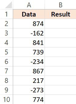
Assume you have the dataset as follows:

The equation that will turn negative integers into positive ones while leaving the remainder untouched is shown below:

=IF(A2>0,A2,-A2)

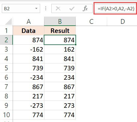
The IF function is used in the formula above to determine if the integer is positive or not first. If the reference is positive, the sign is left alone; if it is negative, a negative sign is added, leaving us with just a positive number.

If the dataset also contains text values, this method will disregard those (and only negative values will be changed)

Once you’ve obtained the desired outcome, you may translate these formulas into values (and copy the original data over in case you don’t require it).

2. Convert all negative numbers to positive ones using the ABS function.

There is a specific function in Excel that removes the minus sign and returns the absolute number.

the ABS component

Let’s say you wish to convert negative numbers to positive values in the dataset depicted below.

The equation to accomplish this is given below:

=ABS(A2)

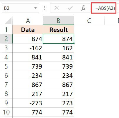
Positive numbers are unaffected by the aforementioned ABS algorithm, however, negative numbers are transformed into positive values.

Once you’ve obtained the desired outcome, you may translate these formulas into values (and copy the original data over in case you don’t require it).

The ABS function has the small limitation of only functioning with numbers. If part of the cells contains text data and you attempt to utilize the ABS function, you will receive a #VALUE! error.

3. Paste Special Multiply to Reverse the Sign

Use this paste-specific multiplication method if you wish to shift the sign of the number from negative to positive or from positive to negative.

Let’s say you have the dataset depicted below and wish to change the sign.

Here are the procedures for using Paste Special to flip the sign:

Enter -1 into any blank cell on the spreadsheet.
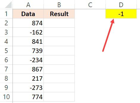
Copied this cell (which has the value -1)
Decide the range you wish to invert the sign for.
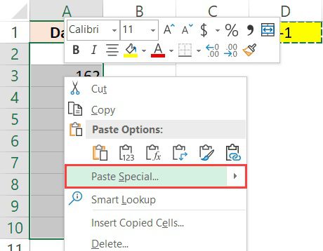
Right-click any of the chosen cells to select it.
Toggle to Paste Special. This will open the Paste Special dialog box
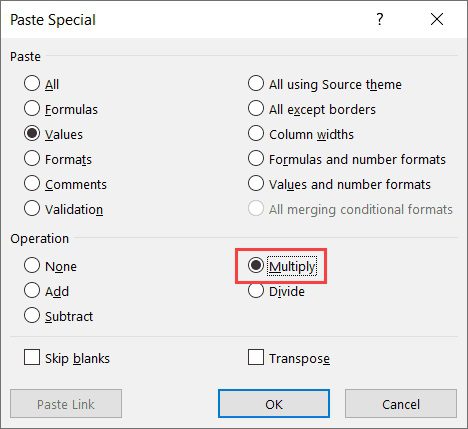
Choose “Values” from the Paste menu.
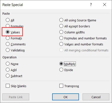
Choose “Multiply” from the Operation choices.
Press “OK”
Subtract -1 from the cell.

You would observe that the aforementioned actions immediately invert the number’s sign (i.e., positive numbers become negative and negative numbers become positive).

What if, however, you simply want to change negative integers into positive ones and not the other way around?

In that scenario, you must first choose all of the negative numbers before continuing with the following procedures.

Here’s how to limit your Excel selection to negative numbers:

Choosing the full collection
Press the F key while keeping the Control key down. The Find and Replace dialogue box will then be shown.
Enter – in the Find What box (the minus sign)
Select Find All.
While maintaining control, hit the A key.

The aforementioned procedures would only choose cells with a negative sign. You may now alter the sign of only the negative values using the Paste Special approach after selecting these cells.

Compared to the formula approach (the two ways discussed before this), this methodology offers the following two advantages:

You don’t have to add a second column and use a formula to populate it with the result. This may be applied to an existing dataset.
The formulae do not need to be changed into values (as the result you get is already a value and not a formula)

4. Remove the Negative Sign With Flash Fill

Flash Fill is a brand-new feature that debuted in Excel 2013.

It enables you to rapidly spot patterns and then provides the outcome after applying the pattern to the complete dataset.

When you have names and wish to distinguish between first name and last name, you may use this technique. Flash Fill will recognize the pattern and offer you all the first names as soon as you input the first name in an adjacent cell a few times.

The positive values of a number can be left untouched while the negative sign is swiftly removed using a similar technique.

I want to convert the negative integers in the dataset below from negative to positive values.

The steps to use Flash Fill to convert negative integers to positive ones are as follows:

Enter the anticipated outcome manually in the box next to the one with the data. In this instance, I’ll manually type 874.
Enter the anticipated outcome in the cell underneath it (162 in this example)
Choose both cells.
Set the cursor above the selection’s bottom right corner. It’ll transform into a + sign.
Drag the mouse to fill the column (or double-click)
Press the AutoFill Options button.
Select Flash Fill.

You would get the desired outcome by following the aforementioned procedures, where the minus sign has been eliminated.

When employing this technique, keep in mind that Excel relies on pattern guessing. Therefore, you must at least inform Excel that you are changing a negative value to a positive one.

This implies that until you have covered at least one negative number, you will need to manually input the intended outcome.

5. Instantly Change Negative Numbers to Positive (VBA)

Last but not least, you may change negative values into positive values using VBA.

If you need to do this frequently, I would advise adopting this technique. Maybe you must do this each time since you frequently obtain the dataset from a coworker or a database.

You may then construct a VBA macro, save it to the Personal Macro Workbook, and add it to the Quick Access Toolbar. So, the following time you receive a dataset where you must do this, all you have to do is choose the data and click the button in the QAT.

… and you’re finished!

Don’t worry; I’ll walk you through every step of setting this up.

The VBA code that will change negative numbers in the chosen range to positive values is listed below:

Sub ChangeNegativetoPOsitive()
For Each Cell In the Selection
    If Cell.Value < 0 Then
        Cell.Value = -Cell.Value
    End If
Next Cell
End Sub

The For Next loop is used in the code above to cycle through each cell in the selection. The IF statement is used to determine whether or not the cell value is negative. The sign is changed if the value is negative; otherwise, it is ignored.

This code may be added to a workbook’s normal module (if you only want to use this in that workbook). Additionally, you may save this macro code in a personal macro workbook for use in any workbook on your system.

The procedures to obtain the Personal Macro Workbook are listed below (PMW).

The steps to preserving this code in the PMW are listed below.

Let me now demonstrate how to include this code in the Quick Access Toolbar (steps are the same whether you save this code in a single workbook or in the PMW)
Open the worksheet containing the data.
the workbook with the VBA code (or to the PMW)
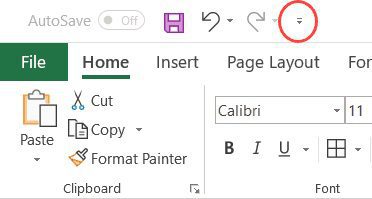
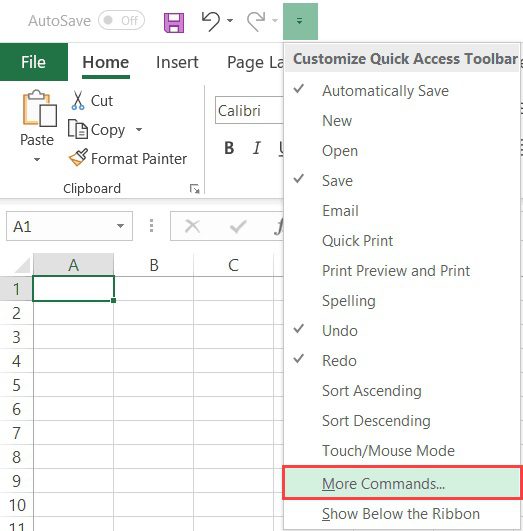
Select “Customize Quick Access Toolbar” from the QA menu.
Select “More Commands”
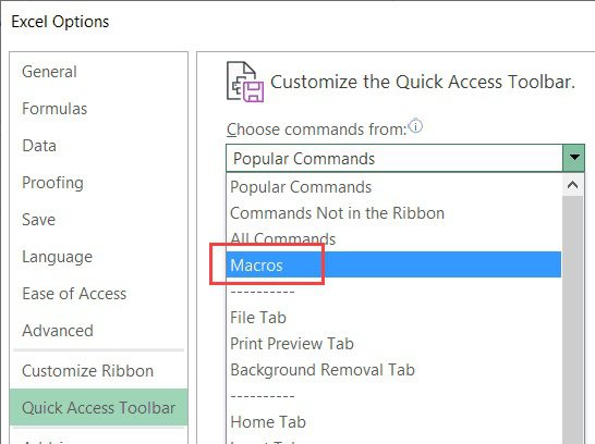
Click the “Choose Commands from” drop-down menu in the Excel Options dialogue box.
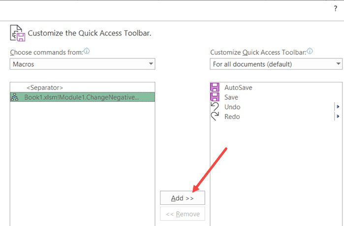
Select Macros. This will display all of the workbook’s macros (or the Personal Macro Workbook)
Press the “Add” button.
OK