What is the best lookup formula in Excel?

VLOOKUP and HLOOKUP are the two lookup operations in Excel that are most frequently used. You can use VLOOKUP to perform a vertical data range search. The HLOOKUP function searches through data structured in rows rather than columns.

How does Hlook up work?

Defines a value in the top row of a table or an array of values, finds it, and then returns a value from the specified row in the table or array in the same column. When Are you Want to look down a specific number of rows, and your comparison values are arranged in a row across the top of a data table, use HLOOKUP Function .

Excel for Office 365 Excel for Mac with Microsoft 365 Excel 2021: Excel for the web

Tip: Use the new XLOOKUP function, an enhanced version of HLOOKUP
that returns precise matches by default and works in either direction,
making it simpler and more practical to use than its forerunner.

This article explains the HLOOKUP function’s syntax and how to use it in Microsoft Excel.

Description
Defines a value in the top row of a table or an array of values, finds it, and then returns a value from the specified row in the table or array in the same column. When your comparison values are in a column to the left of the data you’re looking for, use VLOOKUP.

The H in HLOOKUP stands for “Horizontal.”

Syntax

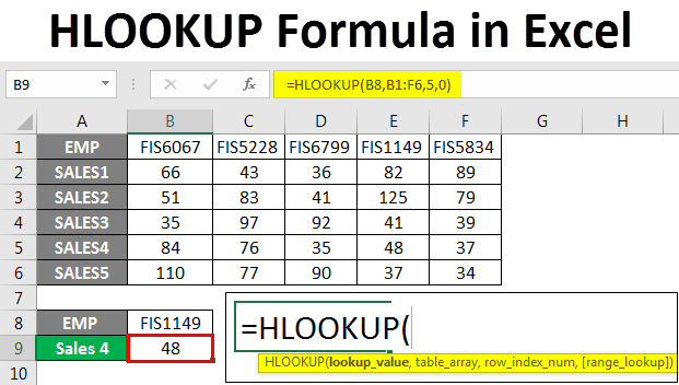
HLOOKUP (lookup value, table array, row index number, [range lookup]) is a syntax.

These arguments are part of the syntax for the HLOOKUP function:

Lookup value

Lookup value Required. the value that can be found in the table’s first row. A value, a reference, or a text string can make up a lookup value.

Table Array

Table array Required. a database table where information is sought. Use a range name or a reference to a range.

Text, numbers, or logical values can all be used as values in the first row of the table array.

The numbers in the first row of the table array must be arranged in ascending order if range lookup is TRUE:…-2, -1, 0, 1, 2,…, A-Z, FALSE, TRUE; otherwise, HLOOKUP might not provide the right result. The table array does not need to be sorted if the range lookup returns FALSE.

both capital and lowercase letters

Text written in uppercase or lowercase is equivalent.

Sort the data from left to right, ascending. See Sort data in a range or table for further details.

Row index NUM

Row index NUM required. The table array row number that the matched value will be returned from. The first-row value in a table array is returned by a row index num of 1, the second-row value is returned by a row index num of 2, and so forth. HLOOKUP returns the #VALUE! Error value if row index num is less than 1, and the #REF! Error value if row index num exceeds the number of rows in the table array.

Range lookup

Range lookup is optional. A logical value indicating whether you want HLOOKUP to look for an exact match. An approximation of a match is returned if TRUE or omitted. In other words, the greatest number that is smaller than the lookup value is returned if an exact match cannot be discovered. HLOOKUP will discover an exact match if FALSE. If none are discovered, #N/A is returned as the error code.

Remark

HLOOKUP utilizes the greatest value that is smaller than the lookup value if the range lookup is TRUE and the lookup value cannot be found.
HLOOKUP returns the #N/A error value if the lookup value is less than the smallest value in the first row of the table array.
You can use the wildcard characters question mark (?) and asterisk (*) in the lookup value if the range lookup is FALSE and the lookup value is text. Any character can be matched by a question mark, whereas any string of characters can be matched by an asterisk. Put a tilde () before the character you want to find, such as a question mark or an asterisk.

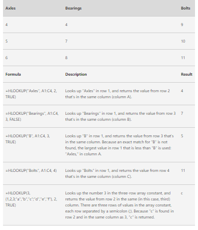
Example

Creating a new Excel worksheet, copy the example data in the accompanying table, then put it in cell A1. Formula results can be seen by selecting them, pressing F2, and then pressing Enter. You can change the column widths if necessary to view all the data.